5 - blockmodeling
The notes below accompany the fifth lecture of the course. It might be a good idea to consult the lecture slides as well, as some technical details and examples are discussed there.
Relational blockmodeling is a distinct approach in network analysis that shifts the focus from analyzing individual nodes or edges to understanding the structural patterns and roles within a network. Unlike classical methods like centrality calculations, which evaluate the importance of individual nodes, or community detection, which identifies cohesive subgroups, blockmodeling examines how actors are grouped based on structural equivalence — the idea that nodes occupying similar positions in a network should display similar patterns of relationships to others. By doing so, it is a generalized approach to analyze network structures as it is not constrained by any specific optimized measure (like density in the Girvan-Newman community detection) or individual focus (like centrality measures).
Developed by Harrison White and further advanced by scholars like Ronald Breiger, Linton Freeman, François Lorrain, and James Moody, among with the many-many other authors, blockmodeling introduced a formal mathematical framework to study how the structure of a network is organized into blocks or positions. This method is particularly suited for identifying underlying roles and patterns that might not be immediately apparent, such as hierarchies, core-periphery structures, or functional differentiation.
Some vocabulary (the list is not complete, though we would not use all of these):
Structural Equivalence: Nodes are structurally equivalent if they have identical relationships to other nodes.
Role Equivalence: A broader concept where nodes have similar, though not identical, roles within the network.
Blocks: Matrix subregions that represent relational patterns between groups of nodes (e.g., dense connections, absence of ties).
Image Matrix: A simplified representation of the network, summarizing relationships between blocks rather than individual nodes.
Fit Function: A measure of how well the blockmodel explains the observed network data.
Relational blockmodeling is particularly powerful for understanding social roles in networks, such as actors in an organization who perform similar tasks or members of a network who share analogous positions (e.g., gatekeepers, brokers). This approach moves beyond individual-level metrics to illuminate the macro-level structure of the network as a whole.
If you want to consult the other sources, check:
recent youtube lecture by James Moody, less than an hour long (it is not focused on coding, though, unlike the other sources),
the structural equivalence chapter from the book Moody and his colleagues wrote (you can also read the chapter 10 “Positions and Roles” in Rawlings et al. (2023), which this linked page accompanies),
the blockmodeling chapter from the other book,
the blockmodeling slides by Anushka Ferligoj,
Phil Murphy & Brendan Knapp post on RPubs on blockmodeling.
The slides I have shown and the code below are partially based on these materials as well.
Libraries for this session:
#########################
## previously covered: ##
#########################

## general:
library(tidyverse)    ## general workflow
library(ggplot2)      ## general for vizualizations
library(ggrepel)      ## captions in ggplot
library(kableExtra)   ## beautiful tables
library(data.table)   ## load csv fast

## for network analysis:
library(igraph)       ## core package to work with networks
library(intergraph)   ## to convert graphs to data frames and back
library(manynet)      ## data package
library(netUtils)     ## to compute network statistics

## data:
library(networkdata)  ## exteremely large library! take time to install in once
#remotes::install_github("schochastics/networkdata") ## installation

########################
## for blockmodeling: ##
########################

#install.packages("concorR")
#devtools::install_github("aslez/concoR")
#install.packages("blockmodeling")
#install.packages("statnet")
#install.packages("sna")

library(concorR)        ## classical package (concor algorithm)
library(concoR)         ## supplementary functions
library(blockmodeling)  ## for signed networks

## general packages, suitable for network analysis in general
## igraph does not allow you to compute these models,
## so we move to the other paradigm of work with networks in R
#library(statnet)
library(sna)
library(FactoMineR)     ## correspondence analysis
library(factoextra)
#remotes::install_version("ggimage", version = "0.3.3")
#library(ggimage) ---> did not work for me for some reasons yeasterday...

#install.packages("ggimg")
library(ggimg)
CONCOR
The CONCOR (CONvergence of iterated CORrelations) algorithm is a classic method in network analysis used to identify groups of nodes with similar structural roles. Developed in the 1970s, it iteratively calculates correlations between the rows (or columns) of an adjacency matrix to group nodes based on their relational patterns. CONCOR is particularly well-suited for blockmodeling and understanding equivalence, as it focuses on similarity in how nodes relate to others rather than direct connections.
This algorithm is often used in contexts like organizational studies or social role analysis, where grouping actors by their patterns of ties provides meaningful insights. Unlike clustering methods based on distance, CONCOR relies on correlations, making it ideal for detecting subtle relational similarities.
To run CONCOR, we first need to get a matrix representation of our network, or stack of matrices if we have data on multiple relations. To start with a simple example, let’s find the roles / blocks / positions in the Big Lebowski(1998) characters’ network. First, we need to get an adjacency matrix:
g <- networkdata::movie_103
#write_rds(g, "datasets/big-lebowski.rds") ## you can get it from github!

data <- networkdata::movie_103 %>%
  as_adjacency_matrix() %>%
  as.matrix()

data[1:5,1:5] ## first 5 rows and columns
#>           ALLAN BARTENDER BLOND MAN BRANDT BUNNY
#> ALLAN         0         0         0      0     0
#> BARTENDER     0         0         0      0     0
#> BLOND MAN     0         0         0      0     0
#> BRANDT        0         0         0      0     1
#> BUNNY         0         0         0      1     0
To apply the CONCOR algorithm, we can simply run concor_hca() function and set the desired number of partitions (p). Note that this function works with lists of martices, meaning we need to put a single matrix inside the list(). The package author’s intention is clearly to run blockmodel when we have multiple ties in our network.
# Apply the CONCOR algorithm:
blks <- concor_hca(list(data), max.iter = 100, p = 2)


## to vizualise, we need to build the block model:
blk_mod <- blockmodel(data,
                      blks$block,
                      mode="graph",
                   #  plabels=blks$vertex,
                      glabels="the Big Lebowski characters",

                      #plabels = rownames(data[[1]]),
                   plabels = V(g)$name
                   )

## see the results:
blk_mod
#>
#> Network Blockmodel:
#>
#> Block membership:
#>
#>        ALLAN    BARTENDER    BLOND MAN       BRANDT
#>            1            1            1            1
#>        BUNNY        CHIEF  CHINESE MAN      DA FINO
#>            1            1            1            1
#>       DIETER     DONNELLY        DONNY       DRIVER
#>            3            1            3            1
#>         DUDE    FIRST MAN        FRANZ         GARY
#>            4            2            3            1
#>      HALLWAY      KIEFFER          MAN        MAUDE
#>            1            3            3            3
#>    OLDER COP        PILAR    POLICEMAN     QUINTANA
#>            1            1            1            3
#>   SECOND MAN       SMOKEY THE STRANGER    THIRD MAN
#>            2            3            1            2
#>         TONY     TREEHORN     WAITRESS       WALTER
#>            1            1            3            3
#>        WOMAN          WOO    YOUNG MAN  YOUNG WOMAN
#>            3            1            1            1
#>  YOUNGER COP
#>            1
#>
#> Reduced form blockmodel:
#>
#>   the Big Lebowski characters
#>            Block 1    Block 2    Block 3   Block 4
#> Block 1 0.04329004 0.00000000 0.02892562 1.0000000
#> Block 2 0.00000000 1.00000000 0.09090909 1.0000000
#> Block 3 0.02892562 0.09090909 0.41818182 0.9090909
#> Block 4 1.00000000 1.00000000 0.90909091       NaN
The function output contains (1) block membership (you can think of it as any other output we got in this course - membership in communities, degree, etc., - it is just a calculated attribute for our nodes), (2) image matrix. To get the image matrix separately, we can run:
round(blk_mod$block.model, 2)
#>         Block 1 Block 2 Block 3 Block 4
#> Block 1    0.04    0.00    0.03    1.00
#> Block 2    0.00    1.00    0.09    1.00
#> Block 3    0.03    0.09    0.42    0.91
#> Block 4    1.00    1.00    0.91     NaN
We can now plot the whole block model:
plot(blk_mod, main = "Big Lebowski blockmodel")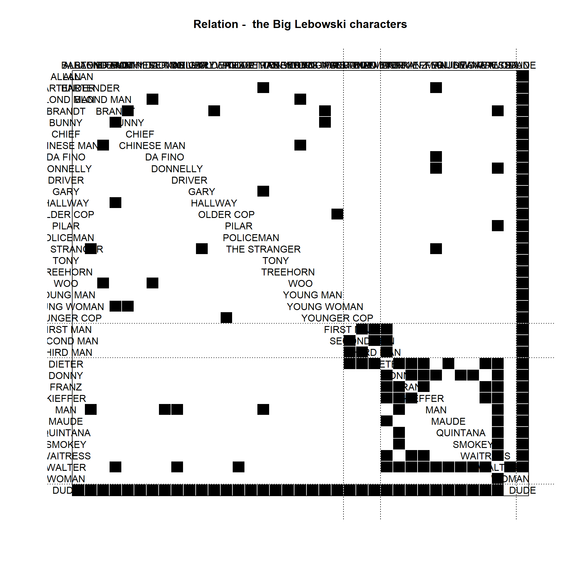
Though it is not an accurate image due to the number of nodes and overlapping names, we can distinguish core/peripherial characters and the main character, dude, who has connection to all the other characters thus constituting a special “role” in the film. In addition to the network topology (core/periphery or community structure, if you want to distinguish first-second-third men as a separate group), we get the approximate “role” (as set of relations) split in the movie.
Here is a way to beautify the matrix:
library(RColorBrewer)

column_cols <- c("grey60", "lightblue", "darkgreen", "coral1")

heatmap(blk_mod$blocked.data,
        Rowv = NA,
        Colv = NA,
        revC = T,
        col = colorRampPalette(brewer.pal(6, "Blues"))(25),
        ColSideColors = column_cols[blk_mod$block.membership],
        RowSideColors = column_cols[blk_mod$block.membership])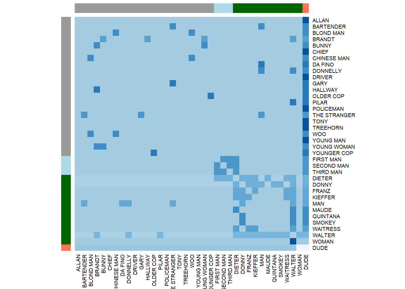
Note that the network we are working with is weighted, so some of the ties are darker than the others.
When plotted on the network, it looks like this:
g <- networkdata::movie_103
V(g)$blocks <- blks$block

set.seed(32)
par(mar=c(0,0,0,0))
plot.igraph(g,
            vertex.color=V(g)$blocks,
            vertex.size = 10,
            edge.color = "grey60",
       edge.width = 2,
       vertex.label = ifelse(igraph::degree(g) > 5,
                             V(g)$name,
                             NA),
       layout = layout_with_mds(g),
       vertex.label.size = 5,
       vertex.label.color = "black")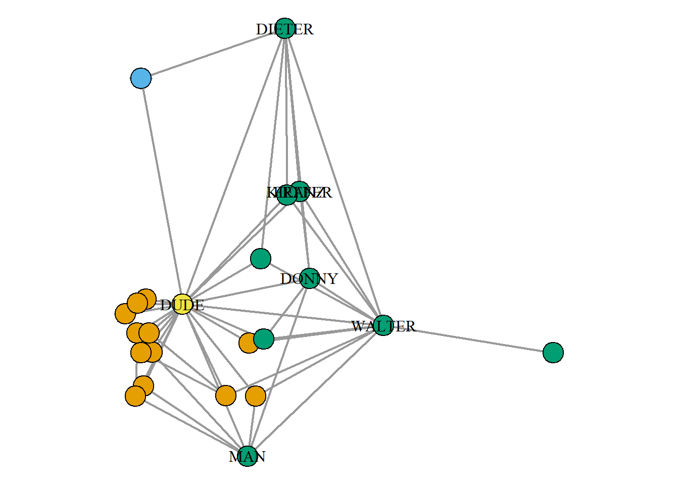
So, the dude has a special role, and there are 3 other blocks of characters.
Regular equivalence with cluster analysis
Next, we would run the other blockmodeling algorithm on the projection of the network we discussed last week. It comes comes from the famous study conducted by Davis and his colleagues (1941). It represents attendance data from 14 social events hosted by 18 women in the American South during the 1930s. This bipartite network captures the affiliations between women and events, highlighting patterns of social interaction, group formation, and shared affiliations. Again, we will work with just one of the projections.
## load the data in appropriate format
bimod.matrix <- southern_women %>%
  as_biadjacency_matrix()

## 2. get the projections by matrices multiplications:

women_matrix <- bimod.matrix %*% t(bimod.matrix)
event_matrix <- t(bimod.matrix) %*% bimod.matrix
## the order of multiplication is important!

## remove the artificial loops:
diag(women_matrix) <- 0
diag(event_matrix) <- 0

## 3. structure of the new one-mode women network:
#women_matrix %>%
#  graph_from_adjacency_matrix(mode = "undirected")

## get igraph objects:
g.women <- women_matrix %>%
  graph_from_adjacency_matrix(mode = "undirected",
                              weighted = T)
## calculate simple centralities:
V(g.women)$degree = igraph::degree(g.women, mode = "all")

## plotting:
par(mar=c(1,1,1,1))
set.seed(32)
g.women %>%
  plot(vertex.label.cex = 0.5,
       vertex.label.color = "black",
       vertex.size = V(g.women)$degree,
       vertex.color = "coral1",
       vertex.shape = "square",
       layout = layout_with_dh(g.women),
       main = "women projection")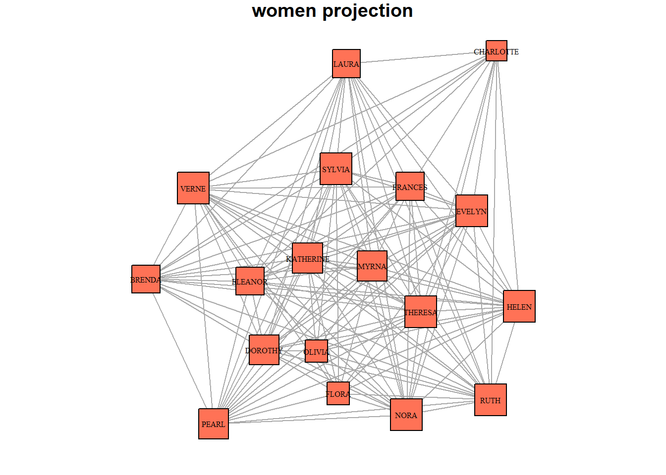
After getting the projection, we delete the weight of the nodes (as opposed to the previous example) and create the matrix object:
g.women2 <- delete_edge_attr(g.women, 'weight')
mat <- as.matrix(get.adjacency(g.women2))
Next, we have 2 options:
equiv.clust()function comes from thesnapackage and produces the solution with so-called approximate equivalence (something in-between structural equivalence and regular equivalence),REGE.ownm.for()function comes from theblockmodelingpackage and produces the solution with regular equivalence.
Let’s first look at the approximate equivalence. We literally ask an algorithm to run the hierarchical clustering on the matrix at hand:
# automorphic equivalence
eq <- equiv.clust(mat,method="euclidean",mode="graph") # specify "graph" for undirected graphs, or "digraph" for directed graphs

plot(eq, labels=eq$glabels)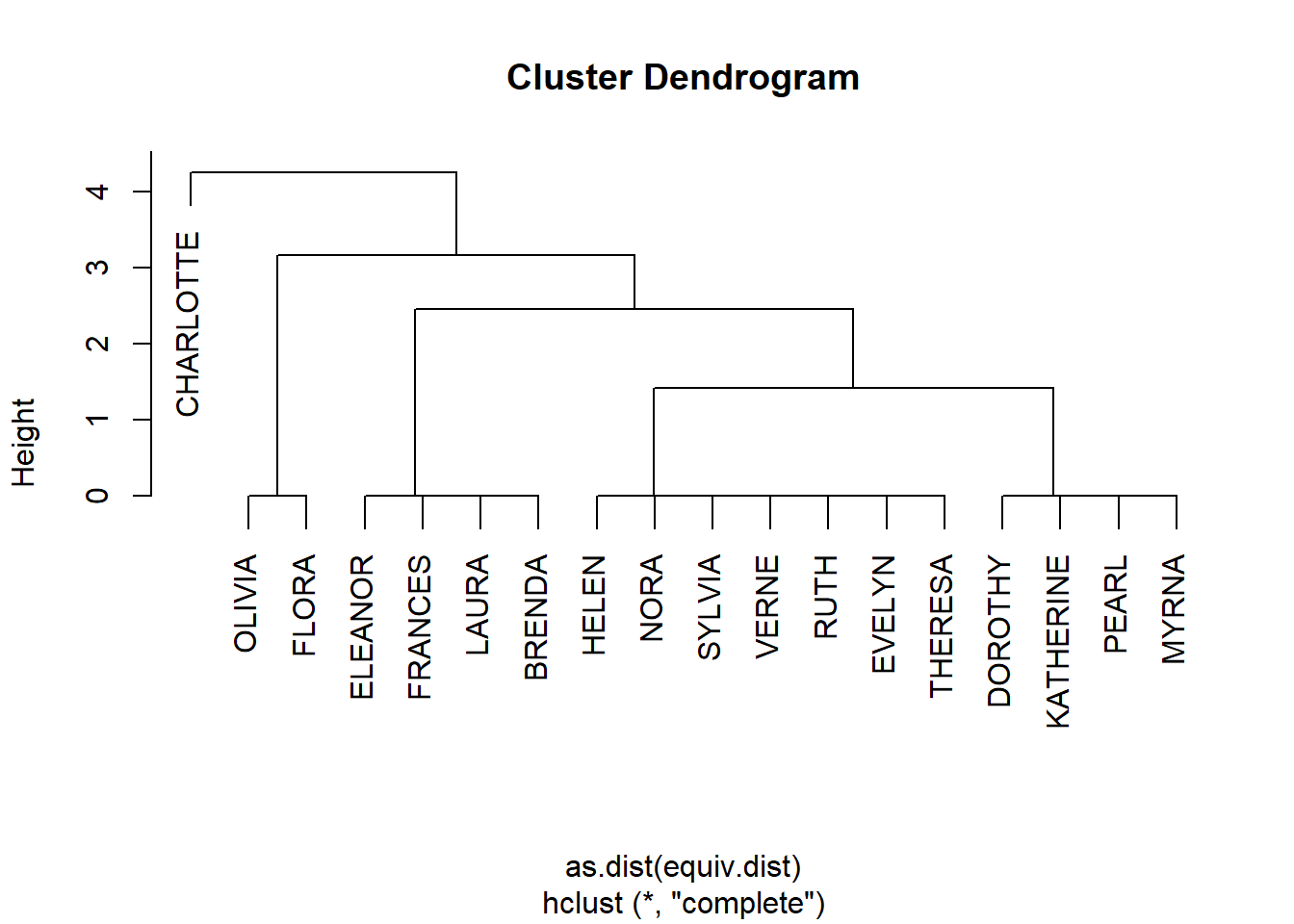
b <- blockmodel(mat, eq, k = 3, mode = "graph") # how many splits to produce (k)If you recall the previous class, there are familiar couples of closely positioned women (Olivia and Flora, for example). Charlotte is early clustered away, meaning she is really distinct from the others. In the context of this research, we can say that she attended the gatherings with a pattern distinct from the rest of the sample (probably, these other groups of women agreed to come to certain events).
Second, regular equivalence:
# regular equivalence

#install.packages("blockmodeling", dependencies=TRUE)
#library(blockmodeling)

#?REGE.ownm.for

REGE.cat <- REGE.ownm.for(M=mat)$E
REGE.part2 <- optRandomParC(M=REGE.cat,
                            k=3, # k = number of subgroups we want to find
                            rep=10,
                            approaches = "hom",
                            homFun = "ss",
                            blocks="com",
                            printRep = F)
#>
#>
#> Optimization of all partitions completed
#> 1 solution(s) with minimal error = 0.07968413 found.

V(g.women)$REGE.class <- REGE.part2$best$best1$clu ## assign partition

heatmap(REGE.part2$M,
        #blk_mod$block.model
  #round(blk_mod$block.model, 2),
        Rowv = NA, Colv = NA, revC = T,
        col = colorRampPalette(brewer.pal(6, "Blues"))(25))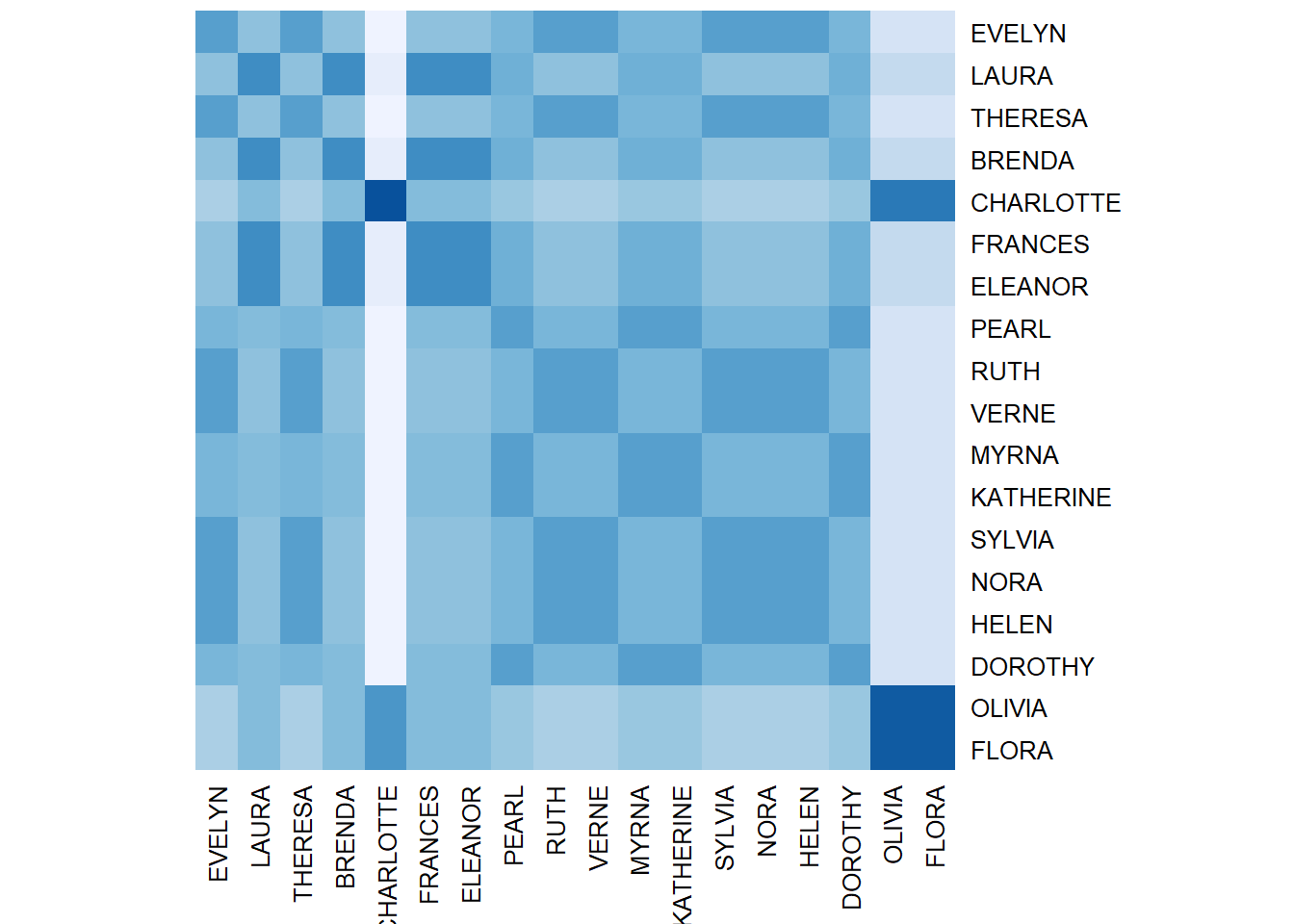
This solution is mode detailed as we can see now the relations between different groups of women and their joint participation in collective life.
Last week network example
It is another portion of blockmodeling on the data we have seen earlier - it is a two-mode network of Russian sociological journals and their (interlocking) editors. I’ll get the journals’ projection and run one of the algorithms from above on it:
## load:
g_journals <- read.csv("datasets/journals_edges.csv") %>%
  graph_from_data_frame(directed = F,
                        vertices = read.csv("datasets/journals_nodes.csv"))

## community detection:

set.seed(42)
cl3 <- cluster_louvain(g_journals,
                       resolution = 0.75)

V(g_journals)$cl3 = membership(cl3)
V(g_journals)$degree = igraph::degree(g_journals, mode = "total")


## solution preview:
set.seed(42)
par(mar=c(0,0,0,0))
plot(g_journals,
     vertex.color = ifelse(V(g_journals)$cl3 == 1,
                           "#988F2A",
                           ifelse(V(g_journals)$cl3 == 2,
                                  "coral1",
                                  "#30638E")),
     vertex.label = NA,
     vertex.size = V(g_journals)$degree * 0.6)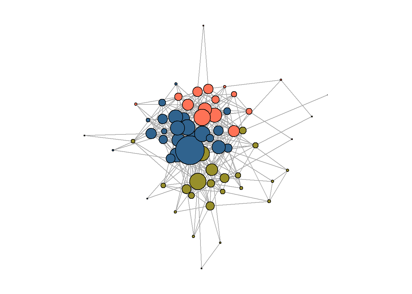
Blocks?
# automorphic equivalence
mat <- as.matrix(get.adjacency(g_journals))

# journal partition in blocks:
#(asDF(g_journals))$vertex %>%
#  group_by(blocks) %>%
#  summarise(journals_included = toString(journal_name)) %>%
#  kable() %>%
#  kable_styling(full_width = F)

eq <- equiv.clust(mat,method="euclidean",mode="graph")
b <- blockmodel(mat, eq, k = 3, mode = "graph",
                glabels = "Russian sociology journals",
                plabels = V(g_journals)$name)


column_cols <- c("grey60", "lightblue", "coral1")


heatmap(b$blocked.data,
        col = colorRampPalette(brewer.pal(3, "Blues"))(25),
        ColSideColors = column_cols[b$block.membership],
        RowSideColors = column_cols[b$block.membership])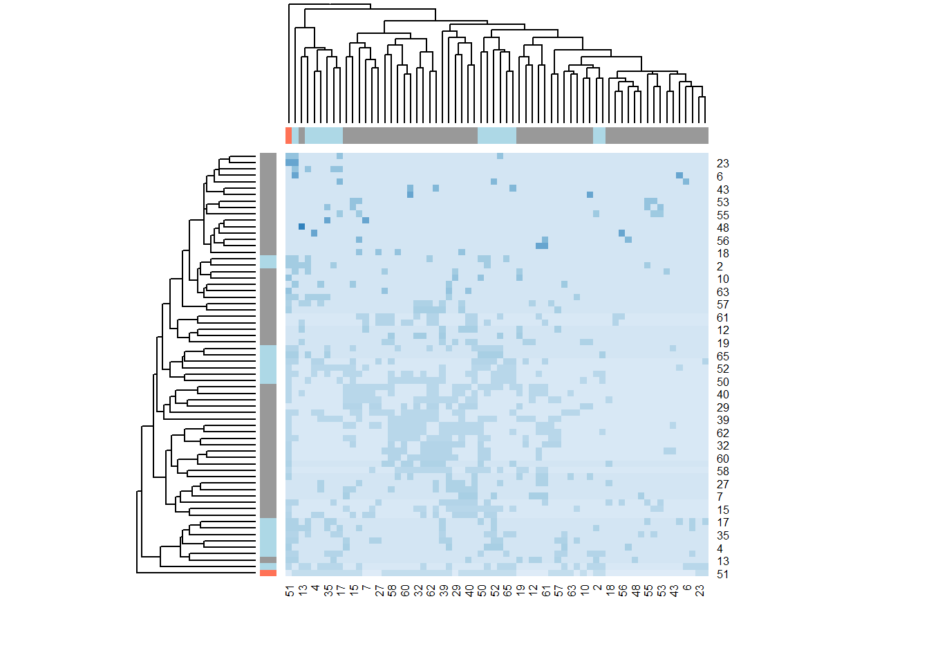
Let’s compare the community detection results with the blockmodeling solution:
V(g_journals)$block = b$block.membership

(intergraph::asDF(g_journals))$vertex %>%
  select(journal_name, cl3, block, degree) %>%

  count(cl3, block)
#>   cl3 block  n
#> 1   1     1 22
#> 2   1     2  4
#> 3   2     1 13
#> 4   2     2  3
#> 5   3     1 15
#> 6   3     2  8
#> 7   3     3  1
The first two clusters include nodes of two types: those from the first and the second blocks. The third cluster contains all roles presented in the network: the single node, “Sociological Research” journal, is the true central node that even gets a separate block.
Again, combining these algorithms can give us insightful results, though sometimes blockmodeling can mirror the more typical network clustering solutions.
V(g_journals)$block <- b$block.membership

new_nodelist <- (intergraph::asDF(g_journals))$vertex %>%
  left_join((intergraph::asDF(g_journals))$vertex %>%
  select(journal_name, cl3, block, degree) %>%

  count(cl3, block) %>%
  mutate(joined.cluster.block = c(1:7)) %>%
  select(-n))

set.seed(42)
par(mar=c(0,0,0,0))

g_journals %>%
  get.edgelist() %>%
  data.frame() %>%
  graph_from_data_frame(directed = F,
                        vertices = new_nodelist) %>%

  plot(vertex.color = V(.)$joined.cluster.block,
       vertex.label = NA,
       vertex.size = V(.)$degree/3)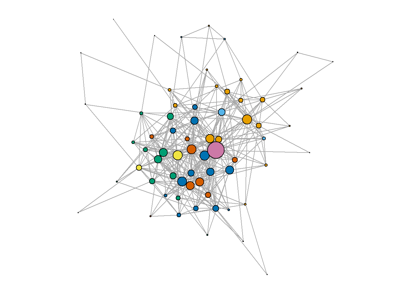
INSNA teacher-student network - a tribute to Harrison White
Data description from the package networkdata:
When Barry Wellman founded the International Network for Social Network Analysis (INSNA) in 1977, he sent a questionnaire to all the founding members. Included were questions on who taught each founder and who each founder taught. This data set is based on their responses.
#?networkdata::insna

insna <- insna
#write_rds(insna, "insna.rds")
insna <- read_rds("datasets/insna.rds")
This network:
contains 60 nodes and 94 directed edges,
describes the relations among the founding figures in the International Network for Social Network Analysis (INSNA) in 1977, - literally, who taught whom and who learned from the basics of SNA.
## centrality measures:
## --------------------
V(insna)$outdegree = igraph::degree(insna, mode = "out")
V(insna)$totaldegree = igraph::degree(insna, mode = "total")

## highlighting Harrison White:
## ----------------------------
edges <- insna %>%
  igraph::as_data_frame(what = "vertices") %>%
  mutate(color = ifelse(name == "Harrison White",
                        "coral1",
                        "grey40"))

## plot:
## -----
set.seed(42)
par(mar=c(0,0,0,0))
insna %>%
  plot(
    vertex.label = NA,
    vertex.size = (5 + V(insna)$outdegree*1.3),
    vertex.color = edges$color,
    edge.color = "black",
    edge.arrow.width = 0.6)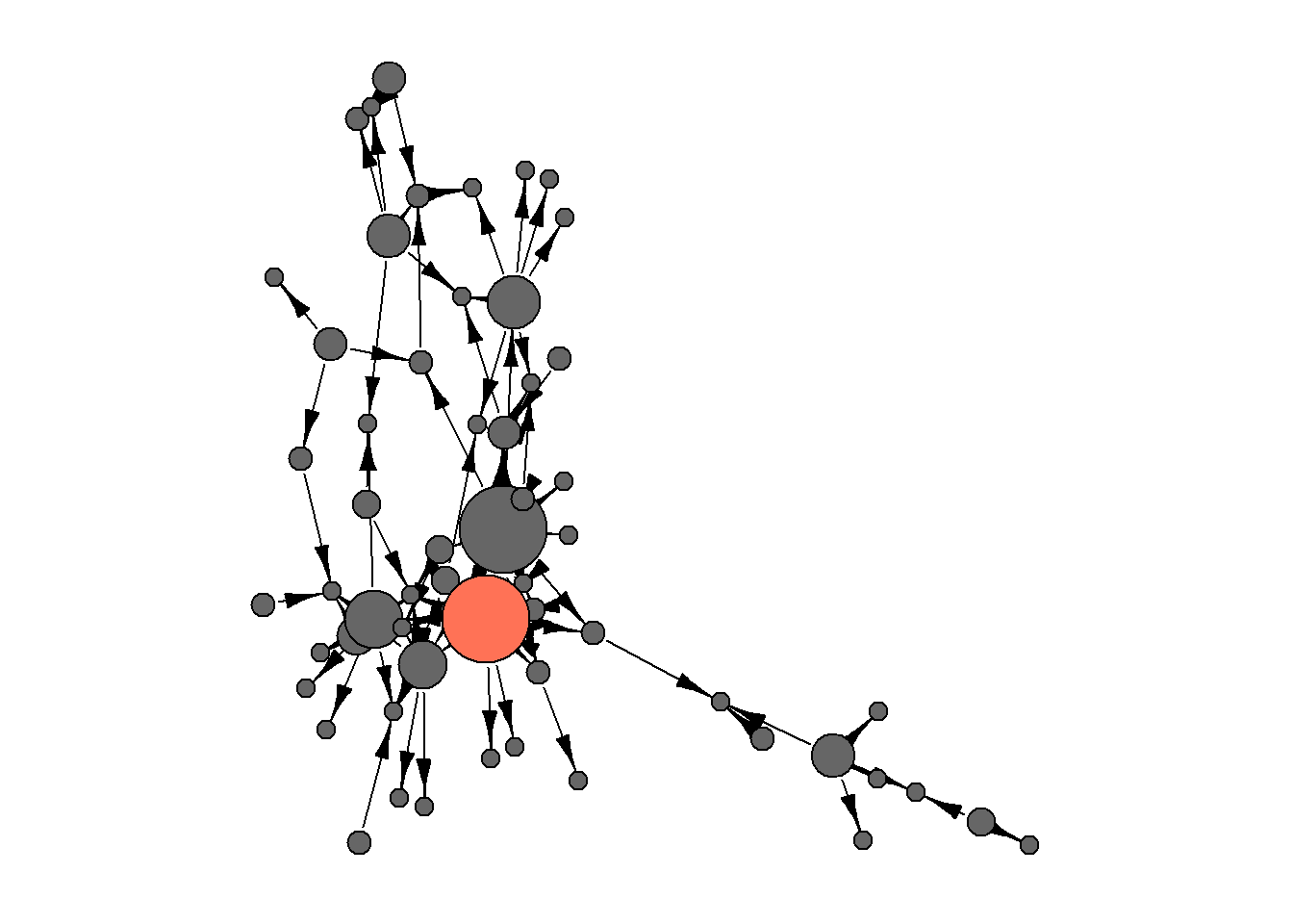
Let’s try to determine the “roles” of each node on this network.
Converting data to matrix form (since the network is directed, we are interested in both the regular matrix and the transposed one; we will use columns as in regular data analysis to calculate correlations/distances):
insna2 <- as_adjacency_matrix(insna,
                              sparse = F)
insna2.1 <- t(insna2)

insna3 <- cbind(insna2,
                insna2.1)
Next, we calculate the distances between nodes, reduce the dimensionality, and see how our authors are ranked:
euclid_dist <- dist(x = insna3,
                   method = "euclidean")

fit <- cmdscale(d = euclid_dist,
                k = 2)

fit %>%
  data.frame() %>%
  mutate(person = row.names(.)) %>%

  ggplot(aes(X1, X2)) +
  geom_text(aes(label = substr(person, 1, 15)), size = 3)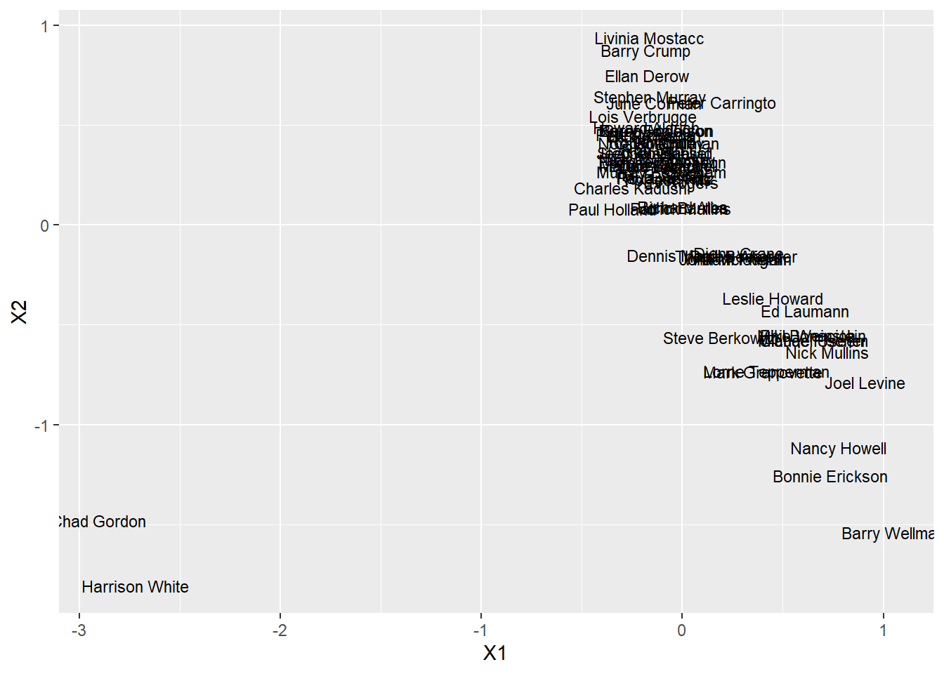
We see on this plot that Chad Gordon and Harrison White are indeed quite distinct from the rest of the network (though there is also some variation on y axis).
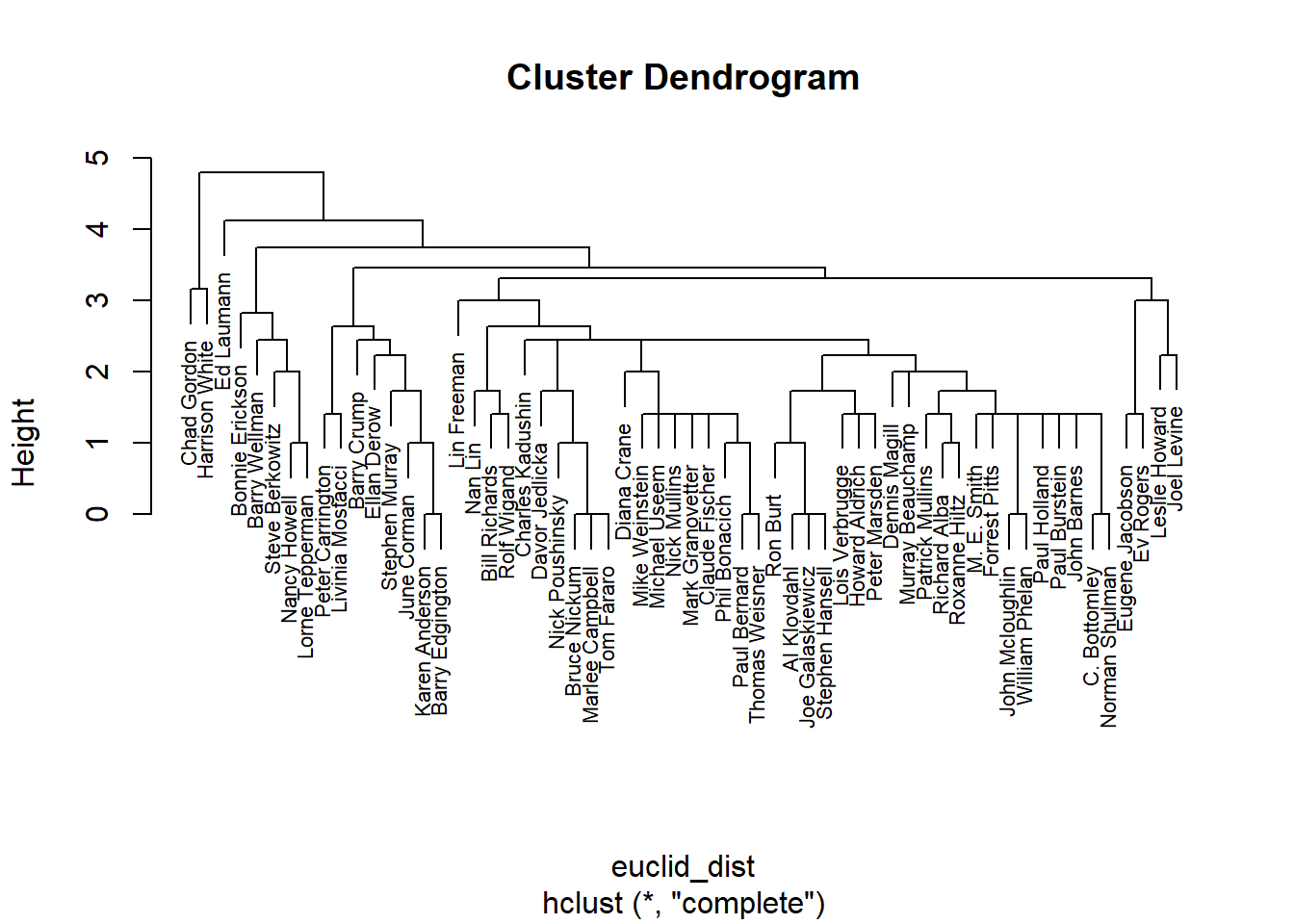
Option for presentation through hierarchical clustering (once again, Gordon and White are quite distinct):
Draw a network with the role coloring (at different degrees of granularity):
V(insna)$roles1 <- cutree(hc, h = 3.8)
V(insna)$roles2 <- cutree(hc, h = 2.5)

par(mfrow = c(1,2))
set.seed(42)
par(mar=c(0,0,0,0))
insna %>%
  plot(
    vertex.label = NA,
    vertex.size = (5 + V(insna)$outdegree*1.3),
    vertex.color = V(insna)$roles1,
    edge.color = "black",
    edge.arrow.width = 0.6,
    main = "\n\nh = 3.8")

set.seed(42)
par(mar=c(0,0,0,0))
insna %>%
  plot(
    vertex.label = NA,
    vertex.size = (5 + V(insna)$outdegree*1.3),
    vertex.color = V(insna)$roles2,
    edge.color = "black",
    edge.arrow.width = 0.6,
    main = "\n\nh = 2.5")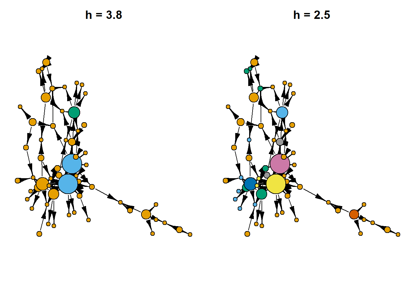
Scaling options
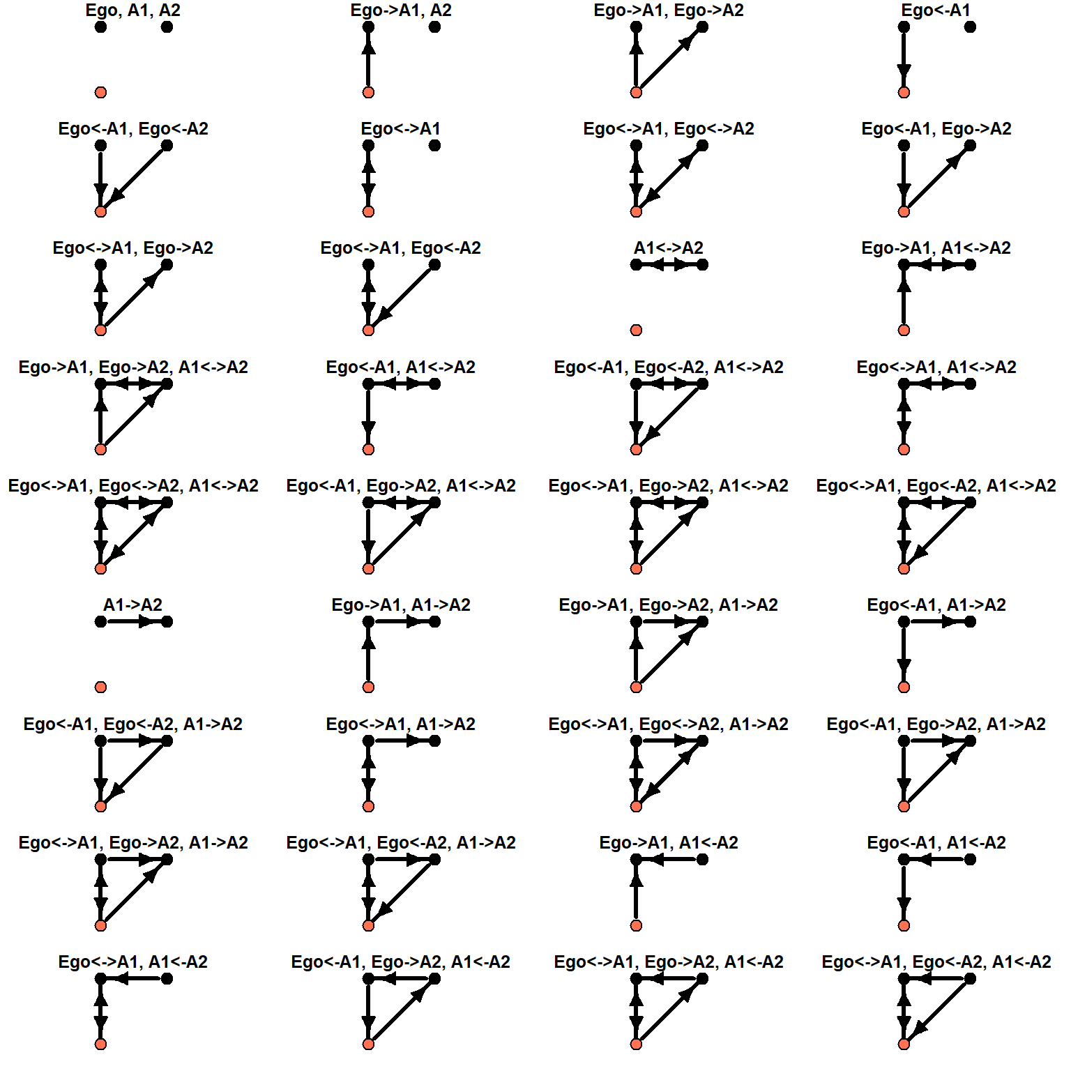
All the triads (16) differentiated by the ego’s positions:
possible.triads <- str_split("1 Ego, A1, A2
2 Ego->A1, A2
3 Ego->A1, Ego->A2
4 Ego<-A1
5 Ego<-A1, Ego<-A2
6 Ego<->A1
7 Ego<->A1, Ego<->A2
8 Ego<-A1, Ego->A2
9 Ego<->A1, Ego->A2
10 Ego<->A1, Ego<-A2
11 A1<->A2
12 Ego->A1, A1<->A2
13 Ego->A1, Ego->A2, A1<->A2
14 Ego<-A1, A1<->A2
15 Ego<-A1, Ego<-A2, A1<->A2
16 Ego<->A1, A1<->A2
17 Ego<->A1, Ego<->A2, A1<->A2
18 Ego<-A1, Ego->A2, A1<->A2
19 Ego<->A1, Ego->A2, A1<->A2
20 Ego<->A1, Ego<-A2, A1<->A2
21 A1->A2 (or A1<-A2)
22 Ego->A1, A1->A2
23 Ego->A1, Ego->A2, A1->A2 (or A1<-A2 )
24 Ego<-A1, A1->A2
25 Ego<-A1, Ego<-A2, A1->A2 (or A1<-A2 )
26 Ego<->A1, A1->A2
27 Ego<->A1, Ego<->A2, A1->A2 (or A1<-A2 )
28 Ego<-A1, Ego->A2, A1->A2
29 Ego<->A1, Ego->A2, A1->A2
30 Ego<->A1, Ego<-A2, A1->A2
31 Ego->A1, A1<-A2
32 Ego<-A1, A1<-A2
33 Ego<->A1, A1<-A2
34 Ego<-A1, Ego->A2, A1<-A2
35 Ego<->A1, Ego->A2, A1<-A2
36 Ego<->A1, Ego<-A2, A1<-A2",
"\\n") %>%
  unlist() %>%
  data.frame(triad = .) %>%
  mutate(id_triad = row.names(.),
         triad = str_remove_all(triad,
                                str_c(row.names(.), " ")))

parse_network_notation <- function(notation) {
  # Split by lines and remove empty lines
  lines <- trimws(unlist(strsplit(notation, "\n")))
  lines <- lines[lines != ""]

  edges <- list()
  all_nodes <- c("Ego")  # Start with Ego as default

  for(line in lines) {
    # Case 1: Just node list (no ties) - "Ego, A1, A2"
    if (!grepl("->|<-|<->", line)) {
      nodes <- trimws(unlist(strsplit(line, ",")))
      all_nodes <- unique(c(all_nodes, nodes))
      next  # No edges to process, move to next line
    }

    # Case 2: Contains edge specifications
    # Split by commas to get individual edge specifications
    edge_specs <- trimws(unlist(strsplit(line, ",")))

    for(edge_spec in edge_specs) {
      edge_spec <- trimws(edge_spec)

      if(grepl("->", edge_spec) && !grepl("<->", edge_spec)) {
        # Directed edge: Ego->A1
        parts <- unlist(strsplit(edge_spec, "->"))
        from <- trimws(parts[1])
        to <- trimws(parts[2])
        edges[[length(edges) + 1]] <- c(from, to)
        all_nodes <- unique(c(all_nodes, from, to))

      } else if(grepl("<-", edge_spec) && !grepl("<->", edge_spec)) {
        # Directed edge: Ego<-A1
        parts <- unlist(strsplit(edge_spec, "<-"))
        from <- trimws(parts[2])  # Reverse direction
        to <- trimws(parts[1])
        edges[[length(edges) + 1]] <- c(from, to)
        all_nodes <- unique(c(all_nodes, from, to))

      } else if(grepl("<->", edge_spec)) {
        # Mutual edge: Ego<->A1
        parts <- unlist(strsplit(edge_spec, "<->"))
        node1 <- trimws(parts[1])
        node2 <- trimws(parts[2])
        # Add both directions for mutual connection
        edges[[length(edges) + 1]] <- c(node1, node2)
        edges[[length(edges) + 1]] <- c(node2, node1)
        all_nodes <- unique(c(all_nodes, node1, node2))
      }
    }
  }

  # Create edge data frame (empty if no edges)
  if(length(edges) > 0) {
    edge_df <- do.call(rbind, edges)
    colnames(edge_df) <- c("from", "to")
  } else {
    edge_df <- data.frame(from = character(), to = character())
  }

  return(list(edges = edge_df, nodes = all_nodes))
}

possible.triads2 <- possible.triads %>%
  mutate(triad = str_remove_all(triad, " \\(or.+"))


par(mfrow = c(9,4))
for(i in c(1:36)){

  g <- parse_network_notation(as.character(possible.triads2[i,1]))

  ## save image to use in plotting later:
  ## ------------------------------------
  png(str_c("images/triadic-pictures/triad-",
            i,
            ".png"),
      width     = 3,
    height    = 3,
    units     = "in",
    res       = 400,
    pointsize = 2,
    bg = "grey")

  g$edges %>%
    graph_from_data_frame(directed = T,
                          vertices = c("Ego", "A1", "A2")) %>%

    plot(vertex.color = c("coral1", "black", "black"),
         edge.color = "black",
         edge.width = 3,
         vertex.size = 50,
         vertex.label = NA,
         edge.arrow.size = 15,
         layout = matrix(c(0,0, 1,0, 1,1), nrow = 3))

  dev.off()

  ## plot here:
  ## ---------
  set.seed(42)
  par(mar=c(1,1,1,1))
  g$edges %>%
    graph_from_data_frame(directed = T,
                          vertices = c("Ego", "A1", "A2")) %>%

    plot(vertex.color = c("coral1", "black", "black"),
         edge.color = "black",
         edge.width = 3,
         vertex.size = 35,
         vertex.label = NA,
         main = str_c(possible.triads2[i,1]),
         layout = matrix(c(1,1, 2,1, 2,2), nrow = 3),
         main.cex = 2,
         edge.arrow.size = 0.8)

}
rm(i, parse_network_notation, possible.triads2, g)Relate to the data.frame for plotting:
possible.triads <- possible.triads %>%
  mutate(path = str_c("images/triadic-pictures/triad-",
                      id_triad,
                      ".png"))
Function introduced by Sodeur & Hummell (1987) and later presented by Burt (1990):
source("https://github.com/JeffreyAlanSmith/Integrated_Network_Science/raw/master/R/f.rc.r")Apply this to just one of the networks:
insna <- read_rds("datasets/insna.rds")

partition.in.triads <- f.rc(insna %>%
       as_adjacency_matrix() %>%
       as.matrix())

head(partition.in.triads %>%
       data.frame())
#>     X1  X2 X3  X4 X5 X6 X7 X8 X9 X10 X11 X12 X13 X14 X15
#> 1 1510  53  0  55  0  0  0  1  0   0   0   0   0   0   0
#> 2 1463   0  0 154  3  0  0  0  0   0   0   0   0   0   0
#> 3 1568   0  0  50  0  0  0  0  0   0   0   0   0   0   0
#> 4 1563  55  0   0  0  0  0  0  0   0   0   0   0   0   0
#> 5 1505 113  1   0  0  0  0  0  0   0   0   0   0   0   0
#> 6 1410 205  6   0  0  0  0  0  0   0   0   0   0   0   0
#>   X16 X17 X18 X19 X20 X21 X22 X23 X24 X25 X26 X27 X28 X29
#> 1   0   0   0   0   0  86   0   0   2   0   0   0   0   0
#> 2   0   0   0   0   0  77   0   0   9   0   0   0   0   0
#> 3   0   0   0   0   0  85   0   0   7   0   0   0   0   0
#> 4   0   0   0   0   0  90   0   0   0   0   0   0   0   0
#> 5   0   0   0   0   0  91   0   0   0   0   0   0   0   0
#> 6   0   0   0   0   0  75   0   0   0   0   0   0   0   0
#>   X30 X31 X32 X33 X34 X35 X36
#> 1   0   4   0   0   0   0   0
#> 2   0   0   5   0   0   0   0
#> 3   0   0   1   0   0   0   0
#> 4   0   3   0   0   0   0   0
#> 5   0   1   0   0   0   0   0
#> 6   0  15   0   0   0   0   0
Run correspondence analysis is utilized to get the 2d-overview of the data (although we lose somewhat 10% of the origianl variance):
ca.results <- CA(partition.in.triads,
                 graph = F,
                 ncp = 5)

#fviz_ca_biplot(ca.results, repel = TRUE)
Plot both triads and individuals (note how we deal with the images produced earlier and employ functions from the package img, which is somewhat long, but at least works for me (ggimage is generally a better choice, but you need to figure out how to load this to R)):
## prepare the data:
## -----------------
plotting.data <- ca.results$row %>%
  data.frame() %>%
  mutate(person = as_data_frame(insna, what = "vertices")$name) %>%
  select(`coord.Dim.1`, `coord.Dim.2`, person) %>%

  bind_rows(ca.results$col %>%
              data.frame() %>%
              select(`coord.Dim.1`, `coord.Dim.2`) %>%
  mutate(id_triad = str_remove_all(row.names(.), "V")) %>%

  left_join(possible.triads) %>%
  mutate(type = "triad-type"))

## plot:
## ----
plotting.data %>%
  ggplot(aes(coord.Dim.1, coord.Dim.2)) +
  geom_point() +

  ## plot images:
  geom_point_img(aes(xmin = coord.Dim.2,
    xmax = coord.Dim.1,
    ymin = coord.Dim.2,
    ymax = coord.Dim.1,
    img = path), size = 0.5) +

  ## plot surnames:
  geom_text_repel(aes(label = person),
            size = 2.2) +

  labs(title = "Triadic inclusion in the INSNA (1978) graph",
       x = "dim-1 (75%)",
       y = "dim-2 (15.7%)") +

  scale_y_continuous(limits = c(-0.5, 3))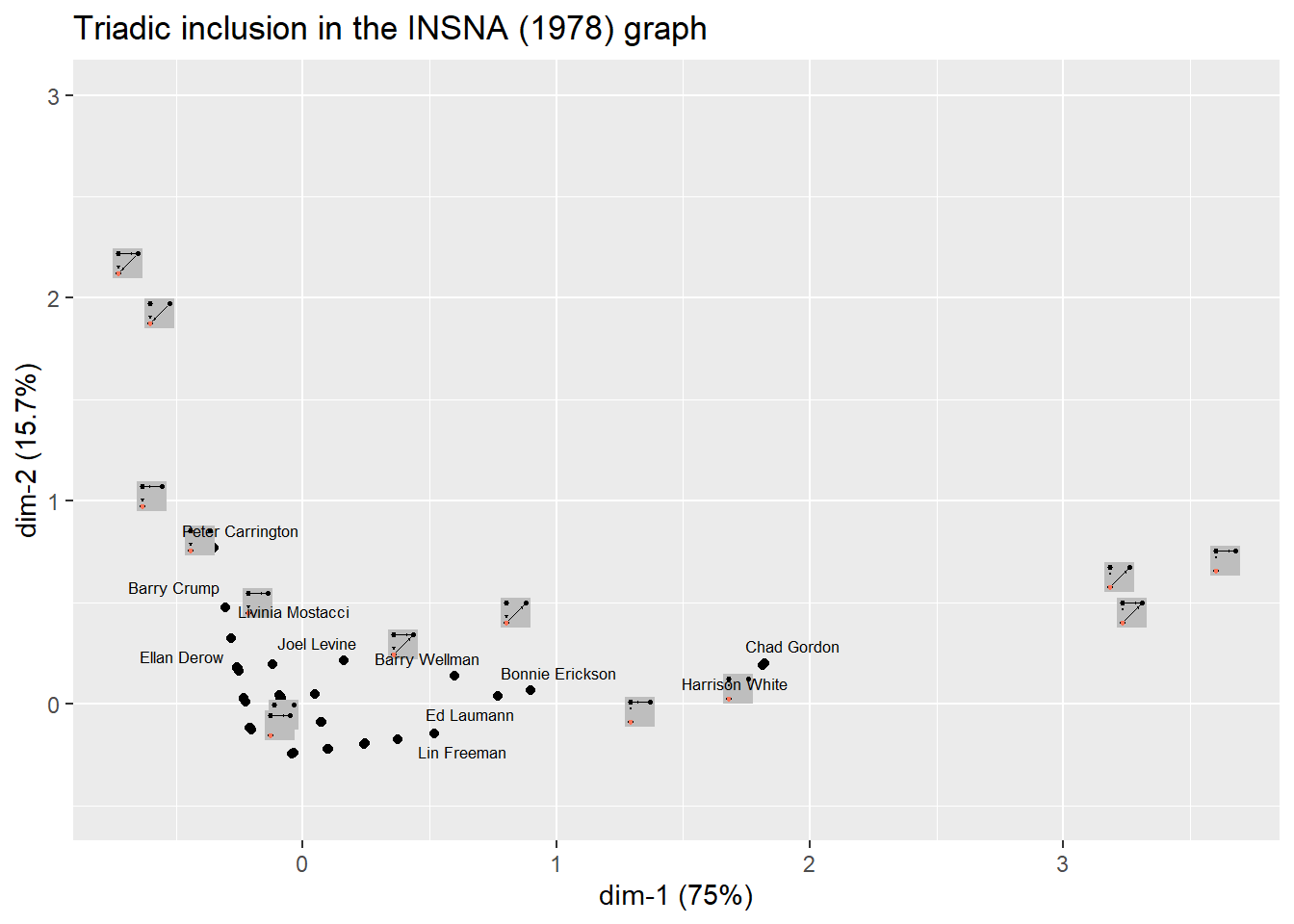
With such a tool & workflow, you can work through dozens of networks (from different time periods or varying organizational contexts) and, through a simple loop, get a second-order clustering of your data, thus checking if there are any coherent and general blocks/roles in these networks.
Read more on the topic in the 10th chapter of:
- Rawlings, C. M., Smith, J. A., Moody, J., & McFarland, D. A. (2023). Network analysis: integrating social network theory, method, and application with R. Cambridge University Press.
Home assignment 5
Choose a dataset you like (preferrably, not very large network – movies’ characters & company dynamics are fine).
describe your data (who are nodes, who are edges, number of both, context, etc.)
run one of the blockmodeling algorithms we discussed in class
does the obtained solution match the nodes’ attributes? (i.e., do variables matter?)
run community detection algorithm you like
compare the results to each other: do they overlap?
Note: to compare communities and blocks, you may need to adjust both solutions (modularity, number of blocks & algorithm selection). Make sure to compare meaningful results from both algorithms. If the results are not overlapping,
- discuss (2-3 sentences, maybe with a picture) how both perspectives are productive when used together.
Submission format: word/pdf/html. If you construct your document from R, make sure it is formatted nicely (no long outputs printed, etc.) Deadline - before your next class.