3 - topology & communities
The notes below accompany the third lecture of the course. It might be a good idea to consult the lecture slides as well, as some technical details and examples are discussed there. During this session, we will:
take a look at graph-level characheristics of the networks,
community detection algorithms,
and learn how to export network data to environments outside R and visualize it. The final section of this page contains notes on sources (we would cover Gephi, GraphCommons, and Cosmograph) and code to prepare your data for the export (mainly, column renaming).
library(tidyverse)
library(igraph)
library(intergraph)
library(manynet)
library(netUtils)   ## for core/periphery
library(netseg)     ## for homphily computation
library(jsonlite)   ## to read hson files

#devtools::install_github("alextkalinka/linkcomm")
library(linkcomm)   ## overlapping communities

# for `networkdata` package:
#install.packages("remotes")
#remotes::install_github("schochastics/networkdata")
## exteremely large library! install if you have 5-7 minutes

library(networkdata)
library(ggplot2)
Graph-level indicators
For this time, we once again will analyze the lawfirm studied by Lazega (2001) available from manynet package. I stack to this example, because it is already familiar to you. Towards the end of this class, we will take a look at other networks.
One-mode network dataset collected by Lazega (2001) on the relations between partners in a corporate law firm called SG&R in New England 1988-1991. This particular subset includes the 36 partners among the 71 attorneys of this firm. Nodal attributes include seniority, formal status, office in which they work, gender, lawschool they attended, their age, and how many years they had been at the firm.
As usual, we load data and split the network into 3 separate networks devoted to the special types of ties:
lawfirm <- ison_lawfirm

nodelist <- (lawfirm %>%
               asDF())$vertexes
edgelist <- (lawfirm %>%
               asDF())$edge

## advice network:
g.advice <- edgelist %>%
  filter(type == "advice") %>%
  graph_from_data_frame(vertices = nodelist,
                        directed = T)

## cowork network:
g.cowork <- edgelist %>%
  filter(type == "cowork") %>%
  graph_from_data_frame(vertices = nodelist,
                        directed = T)

## friendship network:
g.friends <- edgelist %>%
  filter(type == "friends") %>%
  graph_from_data_frame(vertices = nodelist,
                        directed = T)
First, we cover the basic measures to describe the networks.
To explain the diameter measure, I shortly return to karateka network from manynet package to highlight what the measures compute.
karate <- ison_karatekaDiameter is the largest shortest path in the network, the approximate measure of the network’s size. It can be computed with:
get_diameter(karate)
#> + 6/34 vertices, named, from 9e17774:
#> [1] 16     John A 20     Mr Hi  6      17
Here is a (complicated to code) viz of this path:
karate.vertex <- (karate %>%
  asDF())$vertex %>%
  mutate(diameter = ifelse(intergraph_id %in%
                             str_squish(get_diameter(karate)),
                           1,
                           0))


karate.edge <- (karate %>%
  asDF())$edge

karate.edge <- karate.edge %>%
  mutate(edge_couple = str_c(V1, "-", V2)) %>%
  mutate(diameter_edge = ifelse(edge_couple %in% c("16-34",
                                                   #"34-20",
                                                   "20-34",
                                                   #"20-1",
                                                   "1-20",
                                                   "1-6",
                                                   "6-17"),
                                "1",
                                "0"))

set.seed(34)
karate.edge %>%
  graph_from_data_frame(directed = F,
                        vertices = karate.vertex) %>%
  plot(vertex.label = NA,
       vertex.color = ifelse(V(.)$diameter == 1,
                             "coral1",
                             "black"),
       vertex.size = ifelse(V(.)$diameter == 1,
                             20,
                             15),
       edge.width = ifelse(E(.)$diameter_edge == "1",
                             5,
                             1),
       edge.color = ifelse(E(.)$diameter_edge == "1",
                             "coral1",
                             "black"))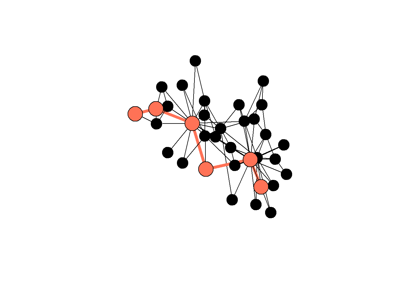
rm(karate1, karate.edge, karate.vertex, karate)
#> Warning in rm(karate1, karate.edge, karate.vertex, karate):
#> объект 'karate1' не найден
And here is a summary table for the types of networks from the lawfirm network. Note the difference between the “cowork” and “friends” networks: the former has a shorter diameter, meaning (1) it is easier for ideas to travel there, (2) this network has more edges in general, so we should interpret the results carefully.
networks <- c("advice",
              "friends",
              "cowork")

diameters <- c(get_diameter(g.advice) %>% length(),
               get_diameter(g.friends) %>% length(),
               get_diameter(g.cowork) %>% length())

n_edges <- c(E(g.advice) %>%
               length(),
             E(g.friends) %>%
               length(),
             E(g.cowork) %>%
               length())

n_vertices <- c(V(g.advice) %>%
                  length(),
                V(g.friends) %>%
                  length(),
                V(g.cowork) %>%
                  length())

#components(g.cowork) - run on different networks

data.frame(networks, n_edges, n_vertices, diameters)
#>   networks n_edges n_vertices diameters
#> 1   advice     892         71         7
#> 2  friends     575         71         8
#> 3   cowork    1104         71         5
Next, let’s discuss centralization and density.
Centralization - the measure of concentration of the network around the nodes with high values of degree centality.
Density - number ob observed ties / number of possible ties. You can interpret it directly, as the measure of number of relations present in the network. Note the maths here: The maximum number of possible edges in a graph can be calculated using the formula \(E_{max} = \frac{n(n-1)}{2}\), where \(n\) represents the number of nodes in the network.
The table below shows these values for our networks:
centralization_scores <- c((centr_degree(g.advice, loops=F))$centralization,
                     (centr_degree(g.friends, loops=F))$centralization,
                     (centr_degree(g.cowork, loops=F))$centralization)

density_scores <- c(edge_density(g.advice),
                    edge_density(g.friends),
                    edge_density(g.cowork)) ## !! note that we cannot compare networks of different size

data.frame(networks,
           centralization = round(centralization_scores,2),
           density = round(density_scores, 2))
#>   networks centralization density
#> 1   advice           0.26    0.18
#> 2  friends           0.18    0.12
#> 3   cowork           0.29    0.22
Next,
Reciprocity - (for directed graphs only) the share of relations which are reciprocal, i.e. directed for both nodes involved.
Transitivity - the density of loops of length three (triangles) in a network, or, in other words, a measure of the nodes’ tendency to cluster together.
Homophily - tendency of the nodes to form ties with similar nodes (similar gender, age, etc.)
Let’s compute these measures for all of our networks (friendship, coworking, advice). For honophily, we check whether nodes tend to be tied to each other based on “gender” or “practice” attributes:
reciprocity_scores <- c(reciprocity(g.advice, mode = "ratio"),
                        reciprocity(g.friends, mode = "ratio"),
                        reciprocity(g.cowork, mode = "ratio"))  # set mode = ratio, it is not by deafult


transitivity_scores <- c(transitivity(g.advice, type = "global"),
                         transitivity(g.friends, type = "global"),
                         transitivity(g.cowork, type = "global")) ## explore local by yourself

homophily_scores <- c(orwg(g.advice %>%
                             simplify(), "gender"),
                      orwg(g.friends %>%
                             simplify(), "gender"),
                      orwg(g.cowork %>%
                             simplify(), "gender"))

homophily_scores.practice <- c(orwg(g.advice %>%
                                      simplify(), "practice"),
                               orwg(g.friends %>%
                                      simplify(), "practice"),
                               orwg(g.cowork %>%
                                      simplify(), "practice"))

#orwg(g.advice %>%
#       simplify(), "practice") ## interpret like odds ratio, “Odds ratio for connected, as opposed to disconnected, dyads depending whether it is between- or within-group, i.e. how much more likely the dyad will be connected if it is within-group.”


data.frame(networks,
           gender.homophily = round(homophily_scores,2),
           practice.homophily = round(homophily_scores.practice, 2),
           reciprocity = round(reciprocity_scores, 2),
           transitivity = round(transitivity_scores,2))
#>   networks gender.homophily practice.homophily reciprocity
#> 1   advice             1.60               3.45        0.24
#> 2  friends             1.62               1.62        0.44
#> 3   cowork             1.33               4.01        0.52
#>   transitivity
#> 1         0.48
#> 2         0.45
#> 3         0.45
Homophily computed in this way requires you to interpret the values like odds ratio, i.e. the chances of establishing a homophilic connection rather than heterophilic one. The function orwg() comes from the “netseg” package.
The core/periphery membership can be estimated as follows (we rely on core_periphery() function from the “netUtils” package):
core_periphery(g.advice)
#> $vec
#>  1  2  3  4  5  6  7  8  9 10 11 12 13 14 15 16 17 18 19 20
#>  0  1  0  1  0  0  0  0  0  0  0  1  1  1  1  1  1  0  1  1
#> 21 22 23 24 25 26 27 28 29 30 31 32 33 34 35 36 37 38 39 40
#>  1  1  0  1  0  1  1  1  1  1  1  1  0  1  1  0  0  0  1  1
#> 41 42 43 44 45 46 47 48 49 50 51 52 53 54 55 56 57 58 59 60
#>  1  1  0  0  0  0  0  0  0  0  0  0  0  0  1  1  0  0  0  0
#> 61 62 63 64 65 66 67 68 69 70 71
#>  0  0  0  0  1  0  0  0  0  0  0
#>
#> $corr
#> [1] 0.3686634
#?core_periphery
Be mindful when using core/periphery detection: many graphs do not exhibit this structure at all. Here is the viz with the solution from above (we need to first assign the computed partition to the nodes):
V(g.advice)$core = core_periphery(g.advice)$vec
V(g.advice)$indegree = degree(g.advice, mode = "in")

g.advice %>%
  as_undirected() %>%
  plot(vertex.label = NA,
       vertex.size = V(g.advice)$indegree/1.5,
       vertex.color = ifelse(V(g.advice)$core == 1,
                             "coral1",
                             "lightblue"))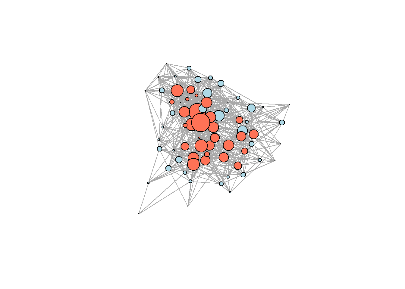
Community detection algorithms
Finally, here is a possible solution to community detection task. Note that it works for undirected graphs, so we need to convert it to undirected mode first like this:
g.friends %>%
  as_undirected()
#> IGRAPH e7981bf UN-- 71 399 --
#> + attr: name (v/c), status (v/c), gender (v/c),
#> | office (v/c), seniority (v/n), age (v/n), practice
#> | (v/c), school (v/c)
#> + edges from e7981bf (vertex names):
#>  [1] 1 --2  1 --4  2 --4  3 --4  3 --7  5 --7  1 --8  4 --9
#>  [9] 2 --10 8 --10 9 --10 4 --11 8 --11 9 --11 10--11 1 --12
#> [17] 2 --12 4 --12 5 --12 8 --12 9 --12 10--12 11--12 4 --13
#> [25] 9 --13 10--13 11--13 12--13 3 --14 4 --14 6 --14 12--15
#> [33] 13--15 2 --16 4 --16 12--16 13--16 14--16 15--16 1 --17
#> [41] 2 --17 4 --17 8 --17 9 --17 10--17 11--17 12--17 13--17
#> + ... omitted several edges
… and here is the community detection function, reproducing the Louvain algorithm (see the lecture slides for details){style=“color: blue;”}:
set.seed(22) ## to reproduce
lc <- cluster_louvain(g.friends %>%
                        as_undirected()) ## !!

V(g.friends)$clusters = membership(lc)

g.friends %>%
  as_undirected() %>%
  plot(vertex.label = NA,
       vertex.size = 10,
       vertex.color = as.character(V(g.friends)$clusters))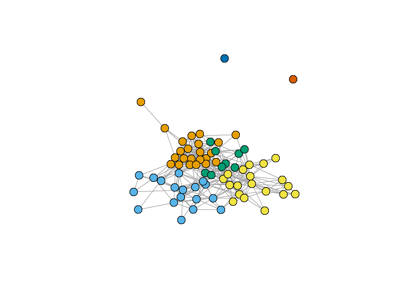
Another important note is that you can use different resolution parameters. Indirectly, it changes the number of communities detected. When applying the algorithm to your data, please, check the whole range of “resolution” values to see how robust your solutions are.
cl0.75 <- cluster_louvain(g.friends %>%
                            as_undirected(),
                       resolution = 0.75)

cl1.75 <- cluster_louvain(g.friends %>%
                            as_undirected(),
                          resolution = 1.75)

V(g.friends)$cl0.75 = membership(cl0.75)
V(g.friends)$cl1.75 = membership(cl1.75)

par(mfrow = c(1,2))
par(mar=c(0,0,0,0))
g.friends %>%
  as_undirected() %>%
  plot(vertex.label = NA,
       vertex.size = 10,
       main = "\n\nresolution = 1.75",
       vertex.color = as.character(V(g.friends)$cl1.75))
par(mar=c(0,0,0,0))
g.friends %>%
  as_undirected() %>%
  plot(vertex.label = NA,
       vertex.size = 10,
       main = "\n\nresolution = 0.75",
       vertex.color = as.character(V(g.friends)$cl0.75))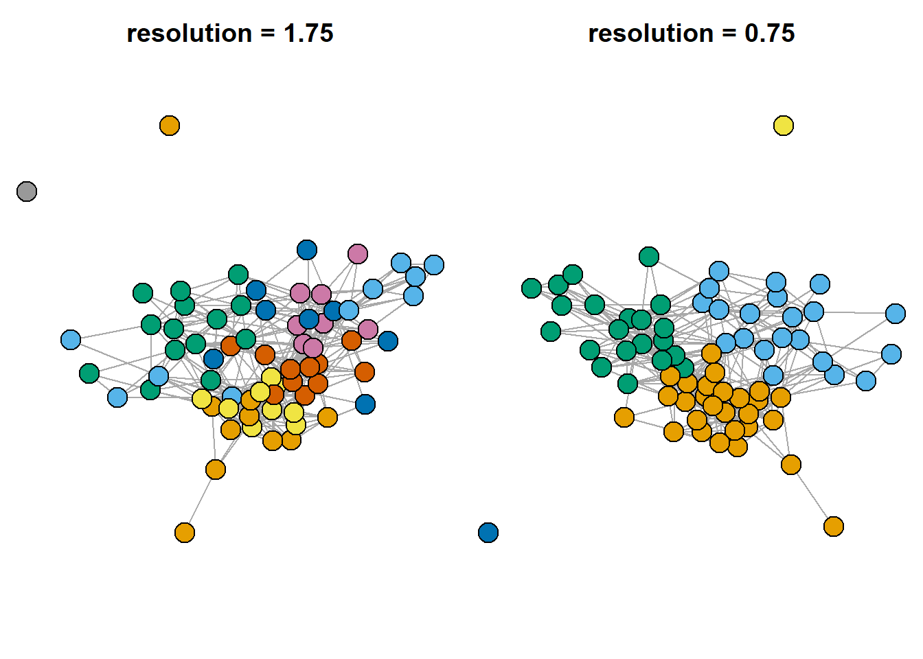
Also, we can search for overlapping communities. I decided not to cover this topic in depth, so, if you are interested, check the “linkcomm” package documentation:
lc <- getLinkCommunities((asDF(g.friends))$edge[,1:2],
                         hcmethod = "single",
                         plot = TRUE, #...or false
                         verbose = F)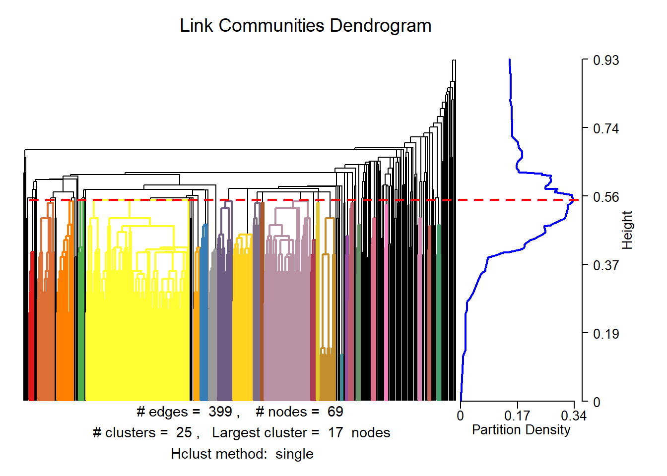
#lc
plotLinkCommGraph(lc,
                  verbose = FALSE)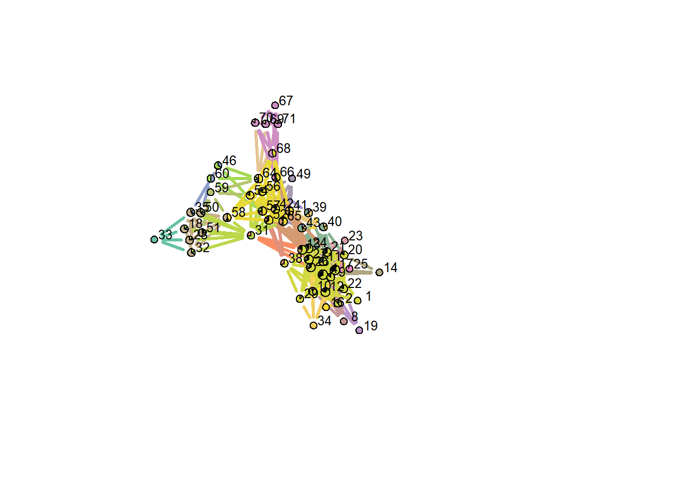
#plot(lc, type = "graph", layout = "spencer.circle")
## see package documentation for more details
Clean environment:
Finally, let’s try to reproduce an image with multiple clustering of karateka dataset (here) - this image is included in the slides, and is intended as an illustration of the idea that there are indeed many approaches to the problem of community detection:
## karateka graph
g <- ison_karateka

## list of basic functions from `igraph` package, without detailed specifications
functions <- list(
  edge_betweenness = function(graph) igraph::cluster_edge_betweenness(graph),
  fluid_comm = function(graph) igraph::cluster_fast_greedy(graph),
  fast_greedy = function(graph) igraph::cluster_fast_greedy(graph),

  infomap = function(graph) igraph::cluster_infomap(graph),
  label_prop = function(graph) igraph::cluster_label_prop(graph),
  ledaing_eigen = function(graph) igraph::cluster_leading_eigen(graph),
  leiden = function(graph) igraph::cluster_leiden(graph),
  louvain = function(graph) igraph::cluster_louvain(graph),
  optimal = function(graph) igraph::cluster_optimal(graph),
  spinglass = function(graph) igraph::cluster_spinglass(graph),
  walktrap = function(graph) igraph::cluster_walktrap(graph))


## plotting parameters:
par(mfrow = c(4,3))

## loop through the functions:
for(i in c(1:11)){

  V(g)$group = functions[[i]](g) %>%
    membership()

  set.seed(1)
  par(mar=c(1,1,1,1))

  g %>%
    plot(vertex.label = NA,
         vertex.size = 12,
         cex.main = 0.8,
         main = functions[i] %>%
           toString() %>%
           str_remove_all("function \\(graph\\) \\n|igraph\\:\\:|\\(graph\\)") %>%
           str_c("()"),
         vertex.color = V(g)$group)
}
#> Warning in igraph::cluster_edge_betweenness(graph): At
#> vendor/cigraph/src/community/edge_betweenness.c:503 :
#> Membership vector will be selected based on the highest
#> modularity score.
Case study: last week OpenAlex network
Last week we have discussed bibliographic networks you can obtain using OpenAlex, an open science source of articles’ metadata and citations’ information. Below is a brief illustration of today’s measures on this network:
library(openalexR)

oa_sustainable <- oa_fetch(entity = "works",
         output = "dataframe",
         display_name.search = 'Sustainable Business Models',
         cited_by_count = ">10",
         verbose = T) ## takes around 20 seconds with my internet connection

oa_edges <- oa_sustainable %>%
  select(id, referenced_works) %>%
  unnest(referenced_works) %>%
  mutate(referenced_works = str_squish(str_remove_all(referenced_works,
                                                      "https\\:\\/\\/openalex\\.org\\/"))) %>%

  filter(referenced_works %in% str_squish(str_remove_all(oa_sustainable$id,
                                              "https\\:\\/\\/openalex\\.org\\/"))) %>%

  mutate(id = str_squish(str_remove_all(id,
                                        "https\\:\\/\\/openalex\\.org\\/"))) %>%
  `colnames<-`(c("from", "to"))

oa_g <- oa_edges %>%
  graph_from_data_frame(directed = T,
                        vertices = oa_sustainable %>%
                          mutate(id = str_remove_all(id,
                                                     "https\\:\\/\\/openalex\\.org\\/")) %>%
                          select(id, title, publication_year, cited_by_count)) %>%
  simplify()

## leave biggest component only

components <- igraph::clusters(oa_g, mode="weak")
biggest_cluster_id <- which.max(components$csize)

# subgraph
oa_g.biggest <- igraph::induced_subgraph(oa_g,
                                         V(oa_g)[components$membership == biggest_cluster_id])

par(mar=c(0,0,0,0))
set.seed(31)
oa_g.biggest %>%
  plot(vertex.label = NA,
       vertex.size = 3,
       vertex.color = "coral1",
       edge.color = "black",
       edge.size = 1,
       edge.arrow.size = 0.5, edge.arrow.width = 0.8)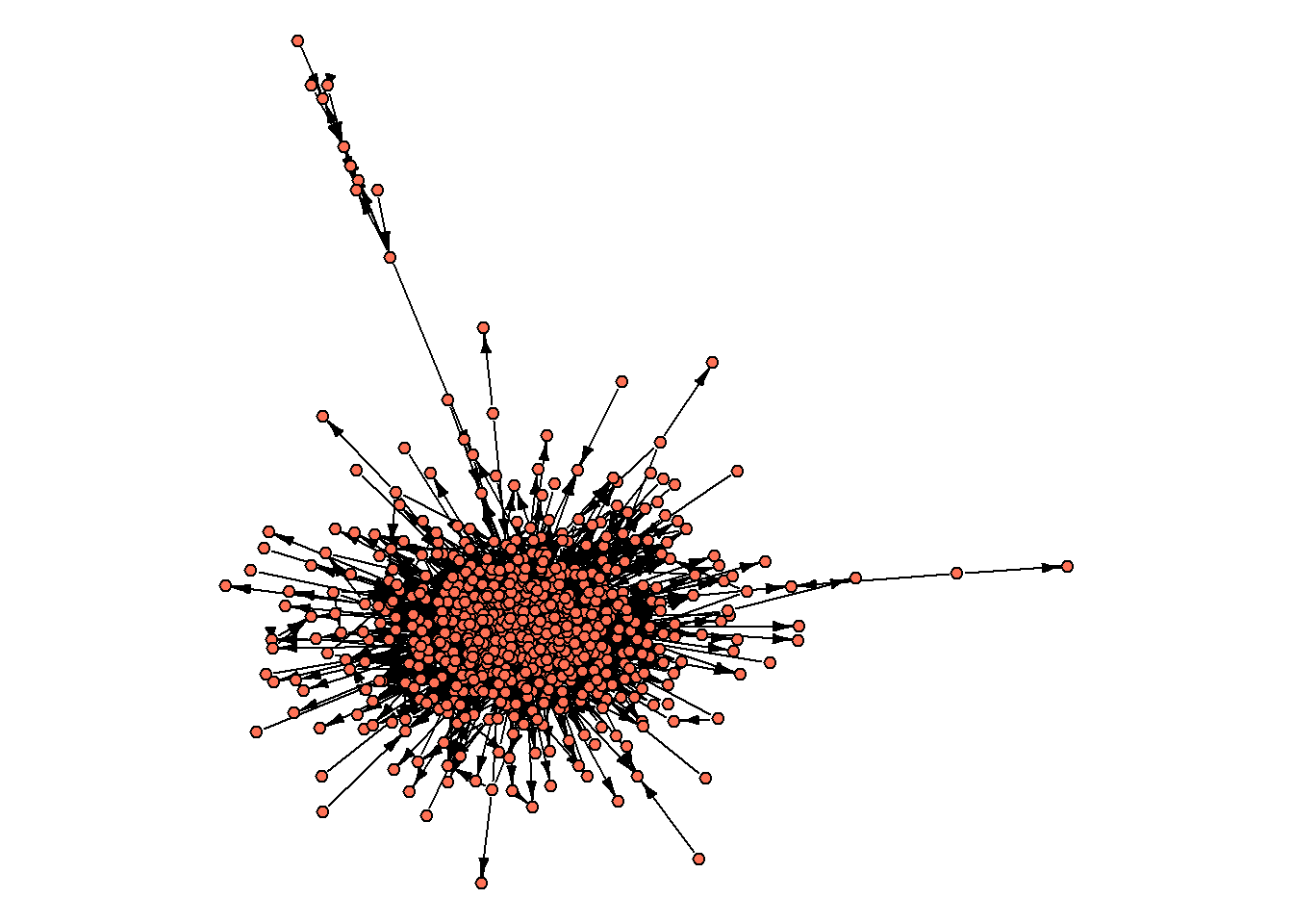
We start by computing the very basic indicators:
diameter(oa_g.biggest) ## 8
#> [1] 8
average.path.length(oa_g.biggest) ## 2.63
#> [1] 2.629412
edge_density(oa_g.biggest %>%
               as_undirected()) ## 0.02
#> [1] 0.02245943
(centr_degree(oa_g.biggest, loops=F))$centralization ## 0.23
#> [1] 0.2329838
Let’s further try to map core/periphery and find communities:
par(mar=c(0,0,0,0))
set.seed(31)
V(oa_g.biggest)$core = core_periphery(oa_g.biggest)$vec
oa_g.biggest %>%
  plot(vertex.label = NA,
       vertex.color = ifelse(V(oa_g.biggest)$core == 1,
                             "coral1",
                             "grey70"),

       vertex.label = NA,
       vertex.size = 3,
       edge.color = "grey70",
       edge.size = 1,
       edge.arrow.size = 0.5,
       edge.arrow.width = 0.8)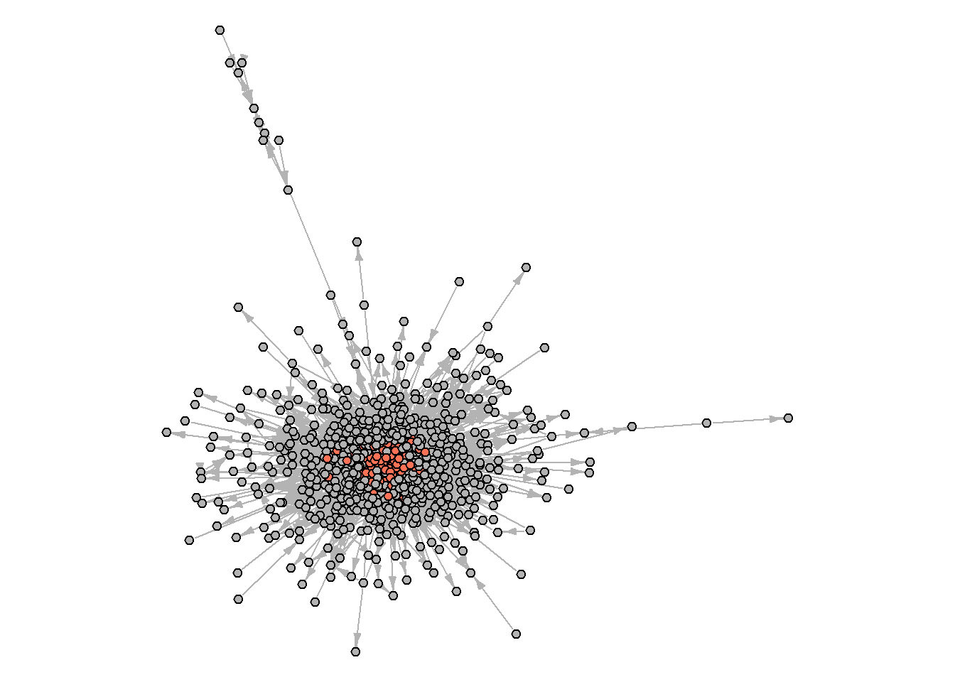
And what about the communities?
set.seed(31)
cl1 <- cluster_louvain(oa_g.biggest %>%
                            as_undirected(),
                          resolution = 0.8)

V(oa_g.biggest)$cl1 = membership(cl1)

par(mar=c(0,0,0,0))
set.seed(31)

plot(oa_g.biggest,
     vertex.label = NA,
     vertex.color = V(oa_g.biggest)$cl1,
            vertex.label = NA,
       vertex.size = 3,
       edge.color = "grey70",
       edge.size = 1,
       edge.arrow.size = 0.5,
       edge.arrow.width = 0.8)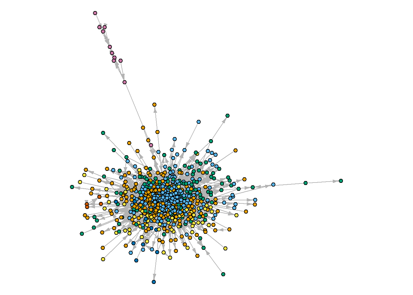
To dive into the obtained clusters, we can group some attributes of the articles to see what’s hidden inside (note that we calculated the share of nodes associated with the “core” coming from each of the calculated communities. In some cases, it might be a good idea, if your communities coexist with the core/periphery structure, - we will cover one such example briefly next time):
(oa_g.biggest %>%
  asDF())$vertex %>%

  #count(cl1) %>%

  group_by(cl1) %>%
  summarise(n = n(),
            share.core = round(mean(core),2),
            mean.age = mean(publication_year, na.rm = T))
#> # A tibble: 7 × 4
#>   cl1            n share.core mean.age
#>   <membrshp> <int>      <dbl>    <dbl>
#> 1 1            219       0.12    2019.
#> 2 2            265       0.27    2019.
#> 3 3            120       0.06    2019.
#> 4 4             69       0.04    2020.
#> 5 5             11       0       2020.
#> 6 6              4       0       2019
#> 7 7             11       0       2014.

#(oa_g.biggest %>%
#  asDF())$vertex %>%

#  ggplot(aes(cited_by_count)) +
#  geom_histogram() +
#  facet_wrap(~as.factor(cl1), scales = "free")
Arguably, we need to adjust our searching query to obtain more meaningful communities, or to use different community detection techniques. At the end of the day, remember, cohesion is easier to measure than to detect communities, and sometimes you do not need to do the latter.
Networks to work in Gephi
Install Gephi first.
In this short tutorial, we’ll look at three datasets in Gephi (available via my github, see the code below, or the course folder) - all sent to you with this code in the archive. Below is a simple example of how to load them into R, analyze them, and save them back for analysis.
insna
The first data set is insna, containing social scientists who studied networks in the 1970s. The data dates back to 1977 and includes information about who taught whom among the participants of the International Network for Social Network Analysis (INSNA). The data was collected by Barry Wellman, the founder of INSNA. Among the 60 participants in the network are Harrison White, Mark Granovetter, Ronald Burt, and Diane Crane.
This data can be obtained from the networkdata package (if you don’t have 5-7 minutes to spare, it’s best not to install this package - it’s very large).
# list all datasets from `networkdata` (987 datasets containing 2260 networks)
## data(package = "networkdata")

# datasets from movies:
## crash <- networkdata::movie_184
## twilight <- networkdata::movie_721

insna <- networkdata::insna

V(insna)$outdegree = degree(insna, mode = "out")
V(insna)$totaldegree = degree(insna, mode = "total")

set.seed(42)
par(mar=c(0,0,0,0))
insna %>%
  plot(vertex.label = NA,
       vertex.size = V(insna)$outdegree*1.5,
       vertex.color = "black",
       edge.arrow.width = 0.3)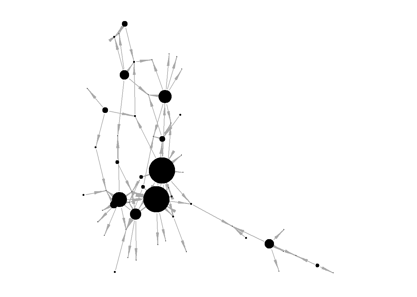
To load lists of edges and nodes, Gephi requires special names for variables:
in the edgelist, the first columns should be named “Source” and “Target”,
in the nodelist, the first columns should be named “Id” and “Label”
This allows Gephi to mark up the data and load everything correctly. In the code below I get the edgelist and nodelist and rename the first columns in them.
insna.edgelist <- (insna %>%
   asDF())$edge %>%
  `colnames<-`(c("Source", "Target"))

insna.nodelist <- (insna %>%
   asDF())$vertex %>%
  rename(Id = intergraph_id,
         Label = name)
Save the data:
# do not forget to check the direction of data saving!
#getwd()

write.csv(insna.edgelist,
          "insna.edgelist.csv",
          row.names = F)
write.csv(insna.nodelist,
          "insna.nodelist.csv",
          row.names = F)
Clear environment:
Twin Peaks (json)
Our next dataset is about the character interactions in “Twin Peaks”. We are interested in this dataset as:
an example of data in an atypical format that can be converted into familiar lists of nodes and edges,
from the point of view of the community search: the data already has clustering, but we will also search for communities in R and look at how to search for communities directly in Gephi.
Load data and look at the network (download json):
Data in the json format is available via archive for today’s class on google drive.
## to read json-files:
# install.packages("jsonlite")


## data loading:
twinpeaks <- fromJSON("datasets/Moviegalaxies - Twin Peaks.json",
                      flatten=TRUE)

## look at the data structure:
#twinpeaks

## edgelist и nodelist:
twinpeaks.edges <- twinpeaks$network$edges
twinpeaks.nodes <- twinpeaks$network$nodes

## create igraph-object:
twinpeaks.g <- twinpeaks.edges %>%
  graph_from_data_frame(vertices = twinpeaks.nodes,
                        directed = F)

## community detection:

set.seed(42)
clustering.louvain <- igraph::cluster_louvain(twinpeaks.g,
                                              resolution = 0.7)

V(twinpeaks.g)$our.louvain <- membership(clustering.louvain)

## create new nodelist:
twinpeaks.nodes2 <- (twinpeaks.g %>%
    asDF())$vertex
What is the intersection of the community detection solutions?
#twinpeaks.nodes2 %>%
#  count(group, our.louvain)

par(mfrow = c(1,2))

set.seed(31)
par(mar=c(1,1,1,1))
twinpeaks.g %>%
  plot(vertex.label = NA,
       vertex.size = 7,
       main = "\noriginal mapping\n")

par(mar=c(1,1,1,1))
set.seed(31)
twinpeaks.g %>%
  plot(vertex.label = NA,
       vertex.size = 7,
       main = "\nlouvain mapping,\nresolution = 0.7",
       vertex.color = ifelse(V(twinpeaks.g)$our.louvain == 1,
                             "coral1",
                             ifelse(V(twinpeaks.g)$our.louvain == 2,
                                    "green",
                                    ifelse(V(twinpeaks.g)$our.louvain == 3,
                                           "blue",
                                           "grey70"))))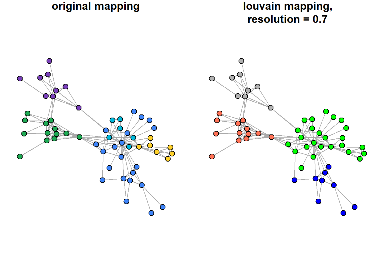
Save data for Gephi:
## note that in the first table the variables are already named correctly, but for the node list we rename and overwrite id:

write.csv(twinpeaks.edges %>%
            rename(Source = source,
                   Target = target),
          "twinpeaks.edgelist.csv",
          row.names = F)
write.csv(twinpeaks.nodes2 %>%
            rename(id = intergraph_id) %>%
            mutate(id = name),
          "twinpeaks.nodelist.csv",
          row.names = F)
Clear the environment:
Dictionary of Russian writers of the 18th century: a network of personalities
Although the authors of the dataset write that “data without preliminary processing can be loaded into programs for network analysis when solving educational problems”, it is still better to firstly observe the files in R to get acquainted with their organization, convert them into a format familiar for work, and calculate the statistics of interest.
Following the authors’ advice, however, we will immediately go to Gephi with this dataset and try to do the entire analysis there.
#list.files() - list files in the directory

writers <- read.table("datasets/Persons_EDGES.tab",
                      header = T)

writers %>%
  head()
#>         Source         Target Weight     Type
#> 1 Н.И.Ахвердов П.И.Богданович      1 directed
#> 2 А.Д.Байбаков     А.А.Барсов      1 directed
#> 3 А.Д.Кантемир     А.К.Барсов      1 directed
#> 4 А.Д.Кантемир    С.С.Волчков      1 directed
#> 5 А.Д.Кантемир  И.И.Ильинский      1 directed
#> 6 А.Д.Кантемир       Ф.Кролик      1 directed
Re-write edges:
write.csv(writers,
          "russian.writers_18century.csv",
          row.names = F)
Data description:
Датасет представляет собой осмысленные в терминах сетевого анализа междустатейные ссылки в Словаре русских писателей XVIII века (1988–2010. Вып. 1–3). Узлами сети выступают посвященные персоналиям статьи словаря, а ребрами – ссылки на другие статьи в том же словаре. Такая сеть позволяет проследить ключевые тенденции в социальном и интеллектуальном взаимодействии литераторов XVIII века.
По словам составителей: «В биографиях лиц, вошедших в историю гуманитарной культуры в качестве государственных деятелей, церковных и светских ораторов, ученых (экономистов, географов, правоведов, историков, лингвистов и пр.), издателей журналов и газет, публицистов, составителей сборников литературного содержания и вместе с тем попадающих в “Словарь”, выделяются и рассматриваются прежде всего сочинения, так или иначе повлиявшие на развитие художественной литературы» (Словарь русских писателей XVIII века. Принципы составления. Словник / сост. В. П. Степанов. Л.: Наука, 1975. С. 11). Таким образом, связи в построенной на данных Словаря сети отражают взаимодействие агентов в поле русской литературы XVIII века.
Data viz from the authors is available here.
If you want, you can also look in Gephi at the second dataset from the same authors, foreign_EDGES.csv, and compare it with the previous data:
Узлами сети выступают русские писатели XVIII века, ребрами — общность их обращения к одним и тем же европейским литераторам. <…> Такая сеть позволяет проследить ключевые тенденции в литературной моде XVIII века. Данные организованы в виде ненаправленного взвешенного графа. Вес ребра означает число общих для данных литераторов упоминаний европейских писателей.
Link to the data (it contains the readme file).
Graph Commons data
For this platform, we need to use different variable names than those required by Gephi. The required renaming is illustrated below with the familiar insna data and the Twin Peaks character network.
For nodes’ list:
“Node Type” (to assign color; I do not use it below)
“Name”
optional: “Description” and “Image”
other columns: anything you want
For edges’ list:
“From Type”
“From Name”
“Edge Type”
“To Type”
“To Name” (“column can have multiple names separated by semicolons for adding multiple connections to these nodes at once.”)
optional: “Weight”
other columns: anything you want
INSNA network:
rm(list = ls())

## load:
insna <- networkdata::insna

## calculate centralities:
V(insna)$outdegree = degree(insna, mode = "out")
V(insna)$totaldegree = degree(insna, mode = "total")

## get edgelist and rename columns appropriately for graph commons:
insna.edgelist <- (insna %>%
   asDF())$edge %>%
  `colnames<-`(c("From Name", "To Name")) %>%
  mutate(`From Type` = "person",
         `Edge Type` = "teaching",
         `To Type` = "person")

## get nodelist and rename columns appropriately for graph commons:
insna.nodelist <- (insna %>%
   asDF())$vertex %>%
  rename(Name = intergraph_id,
         displayed_name = name) %>%
  mutate(`Node Type` = "person")

# check directory:
#getwd()

# save:
write.csv(insna.edgelist,
          "GC.insna.edgelist.csv",
          row.names = F)
write.csv(insna.nodelist,
          "GC.insna.nodelist.csv",
          row.names = F)
“Twin peaks”:
## to read json-files:
# install.packages("jsonlite")
library(jsonlite)

# clear env:
rm(list = ls())

## load data:
twinpeaks <- fromJSON("datasets/Moviegalaxies - Twin Peaks.json",
                      flatten=TRUE)

## edgelist и nodelist:
twinpeaks.edges <- twinpeaks$network$edges
twinpeaks.nodes <- twinpeaks$network$nodes

## re-naming:
twinpeaks.nodes <- twinpeaks.nodes %>%
  select(-id, -color) %>%
  rename(Name = name) %>%
  mutate(`Node Type` = "character")

twinpeaks.edges <- twinpeaks.edges %>%
  rename(`From Name` = source,
         `To Name` = target,
         Weight = weight) %>%
  mutate(`From Type` = "character",
         `To Type` = "character",
         `Edge Type` = "plot connection")

# save:
write.csv(twinpeaks.edges,
          "GC.twinpeaks.edgelist.csv",
          row.names = F)
write.csv(twinpeaks.nodes,
          "GC.twinpeaks.nodelist.csv",
          row.names = F)
Read (more)https://docs.graphcommons.com/ about graph commons.
Cosmograph
This is a free-to-use online tool from the Russian creators. Way more advanced than the previous tools.
Website(https://cosmograph.app/run/){style=“color: blue;”},
The data format needs:
edgelist (“source”, “target”) - it is already enough to build the graph, though you can also add columns “time” and “value”
nodelist = metadata file (“id”, “color”, “size”)
To put your hands on the program, you can load the files about the connections of Russian writers created above into the program: they are already in the appropriate format (source, target), and therefore no modifications are needed.
Home assignment 3
Choose a dataset you like ((check Available datasets) or find a network by yourself), format it appropriately (lists of nodes and edges), and draw the network in Gephi or other software (Graph Commons, Cosmograph). Think about the story you want to tell by showing your network (specific nodes’ positions, network structure, etc.). Feel free to edit the picture using other softwares (if you struggle with captions in Gephi, for example, you can annotate your picture somewhere else).
Insert your graph to pdf/word and write 5-6 sentences about your thought process and story behind the image. Refer to network properties we discussed in class (diameter, homophily, core/peripherical structure) to support your arguments.
If you want to practice more, you can accompany your work with a short report about the most central nodes in the network and/or the structure of the network, including your interpretation of these results.
Deadline: before next class | send to aapecherskikh@hse.ru