4 - two-mode networks
Two-mode networks, or bipartite networks, or affiliation networks (these are used interchangeably sometimes), consist of two distinct sets of nodes, where ties exist only between nodes of different sets (e.g., people and events, authors and papers). This structure is particularly useful for representing affiliations, co-occurrences, or memberships, while preserving the relationships between these categories. Unlike one-mode networks, analyzing two-mode networks requires specialized workflows and metrics to account for their unique structure. In this session, we will walk through the steps of construction, vizualization, and analysis of a two-mode network.
If you want to consult the other sources, check:
this or that pages with the workflow in R. Partially, we will take a look at the data from the first source below.
Today’s lecture slides are available here.
Libraries for this session:
library(tidyverse)    ## general workflow
library(ggplot2)      ## general for vizualizations
library(igraph)       ## core package to work with networks
library(intergraph)   ## to convert graphs to data frames and back
library(manynet)      ## data package
library(netUtils)     ## to compute network statistics

# for `networkdata` package:
#install.packages("remotes")
#remotes::install_github("schochastics/networkdata")

library(networkdata)  ## exteremely large library! take time to install in once

#install.packages("oaqc")
#library(oaqc)         ## for more layouts
#library(graphlayouts) ## for more layouts

#install.packages("tnet")
library(tnet)         ## to analyze 2-mode networks without projections

library(data.table)
library(ggrepel)
library(kableExtra)
library(stringr)
Basic example
The data for the first part of today’s session comes from the famous study conducted by Davis and his colleagues (1941). It represents attendance data from 14 social events hosted by 18 women in the American South during the 1930s. This bipartite network captures the affiliations between women and events, highlighting patterns of social interaction, group formation, and shared affiliations. It is a classical dataset to tell students about the two-mode network analysis.
This data is available via the networkdata package that you should already be aware of. Just in case, this same dataset (in .RData extension) is attached to the zip-folder available via our google drive folder.
# ?southern_women # - to know more aboout the data

## get data from `networkdata`:
data(southern_women)

## save data for it to be available to you
#save.image("southern_women.RData")

## load this same data back:
load("datasets/southern_women.RData")
southern_women %>%
  str()
#> -----------------------------------------------------------
#> UNNAMED NETWORK (undirected, unweighted, two-mode network)
#> -----------------------------------------------------------
#> Nodes: 32, Edges: 89, Density: 0.1794, Components: 1,
#> Isolates: 0
#> -Vertex Attributes:
#>  type(l): FALSE, FALSE, FALSE, FALSE, FALSE, FALSE, ...
#>  name(c): EVELYN, LAURA, THERESA, BRENDA, CHARLOTTE, ...
#> ---
#> -Edges (first 10):
#>  EVELYN--6/27 EVELYN--3/2 EVELYN--4/12 EVELYN--9/26
#> EVELYN--2/25 EVELYN--5/19 EVELYN--9/16 EVELYN--4/8
#> LAURA--6/27 LAURA--3/2
By looking at this data structure, you should note several things:
types of nodes (women and events) are not differentiated when counting the number of nodes.
However, there is a nodes’ attribute “type” which specifies whether a node is an event or a women. When you create a graph with the two-mode organization by yourself,
igraphwould not recognize its special nature unless you provide this variable, “type”, in the nodes’ list.
Let’s try to plot this graph to get a better sense of two-mode networks:
#asDF(southern_women) - run to see how people are distinguished from events

set.seed(42)
par(mar=c(0,0,0,0))
southern_women %>%
  plot(vertex.label.cex = 0.5,
       vertex.label.color = "black",
       vertex.color = ifelse(V(southern_women)$type == FALSE,
                             "coral1",
                             "darkblue"),
       vertex.shape = ifelse(V(southern_women)$type == FALSE,
                             "square",
                             "circle"))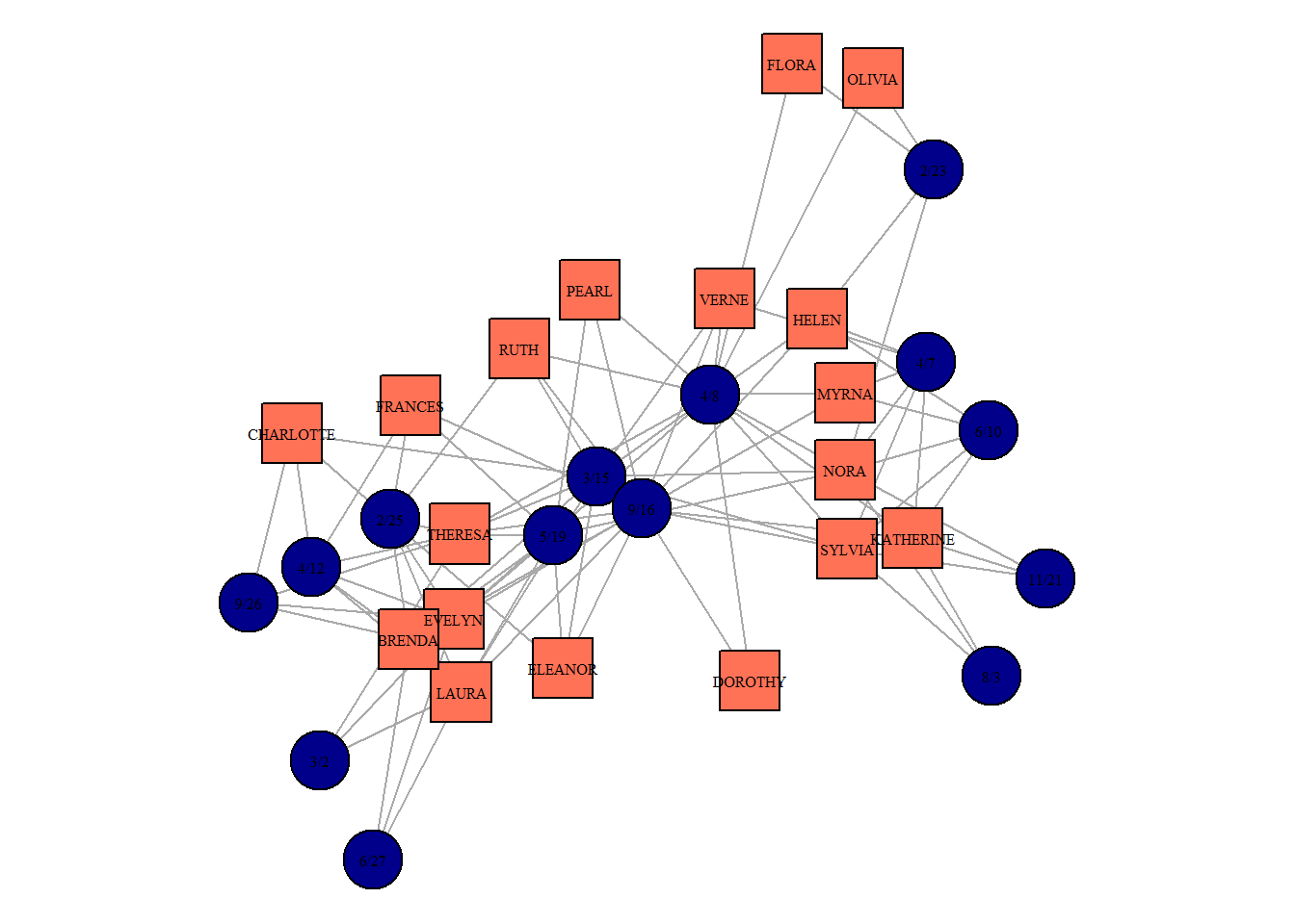
igraph includes some fancy network layouts which can look pretty when dealing with two-mode networks. These examples also show you how to excel at network visualizations in R:
we remove nodes’ captions to simplify the picture,
we code the types of nodes using colors and shapes together,
we change layouts each time to see whether the network structure is presented intuitively clear,
finally, we add titles so that the layout applied is shown.
par(mfrow = c(2,2))
par(mar=c(2,2,2,2))
southern_women %>%
  plot(vertex.label = NA,
       vertex.color = ifelse(V(southern_women)$type == FALSE,
                             "coral1",
                             "darkblue"),
       vertex.shape = ifelse(V(southern_women)$type == FALSE,
                             "square",
                             "circle"),
       layout = layout_as_bipartite(southern_women),
       main = "layout_as_bipartite()")

par(mar=c(2,2,2,2))
southern_women %>%
  plot(vertex.label = NA,
       vertex.color = ifelse(V(southern_women)$type == FALSE,
                             "coral1",
                             "darkblue"),
       vertex.shape = ifelse(V(southern_women)$type == FALSE,
                             "square",
                             "circle"),
       layout = layout_nicely(southern_women),
       main = "layout_nicely()")

par(mar=c(2,2,2,2))
southern_women %>%
  plot(vertex.label = NA,
       vertex.color = ifelse(V(southern_women)$type == FALSE,
                             "coral1",
                             "darkblue"),
       vertex.shape = ifelse(V(southern_women)$type == FALSE,
                             "square",
                             "circle"),
       layout = layout_in_circle(southern_women),
       main = "layout_in_circle()")

par(mar=c(2,2,2,2))
southern_women %>%
  plot(vertex.label = NA,
       vertex.color = ifelse(V(southern_women)$type == FALSE,
                             "coral1",
                             "darkblue"),
       vertex.shape = ifelse(V(southern_women)$type == FALSE,
                             "square",
                             "circle"),
       layout = layout_with_mds(southern_women),
main = "layout_with_mds()") 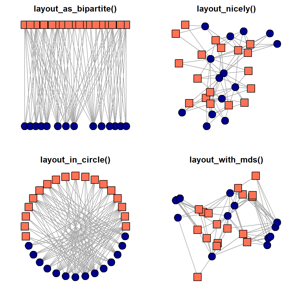
Probably, the core message in-scripted in these pictures is the presence of two types of nodes and the exclusive attachment of dissimilar nodes to each other. Again, these are the core features of the two-mode networks, and they bound the range of techniques we can apply to study this graph.
Theoretically, we have 3 options:
proceed as usual, and apply typical one-mode measures to the two-mode network
analyze each mode separately using two-mode metrics
convert the two-Mode network into two projections (i.e., a network of women and a network of events, where the ties correspond to the omitted type of nodes) and analyze them both as the usual one-mode networks.
The first approach involves treating the two-mode network as-is and applying standard metrics like degree centrality, betweenness centrality, and closeness centrality directly to the bipartite structure. While familiar and straightforward, this strategy may overlook nuances specific to the two-mode context, as many of these measures assume homogeneity among nodes. For example, computing degree centrality can highlight which women attended the most events and which events had the highest participation, meanwhile writing these centrality values into a single column. This last obstacle can puzzle us once the networks get larger and some of the second-order nodes receive too many connections. To put shortly, the comparison of the centralities of these two types of nodes might be misleading. And it gets worse with other measures, and degree centrality, as the simpliest version of centrality, is an only real option to calculate (even with the difficulties just metioned).
V(southern_women)$degree = degree(southern_women,
                                  mode = "all") ## note that affiliation networks cannot be directed, in a sense, as well as its projections

(asDF(southern_women))$vertex %>%
  select(-intergraph_id) %>%
  mutate(type = ifelse(type == F,
                       "women",
                       "event")) %>%
  group_by(type) %>%
  slice_max(degree, n = 3) %>%
  kable() %>%
kable_styling(full_width = F)| type | name | degree |
|---|---|---|
| event | 9/16 | 14 |
| event | 4/8 | 12 |
| event | 3/15 | 10 |
| women | EVELYN | 8 |
| women | THERESA | 8 |
| women | NORA | 8 |
The code from above computes the degree centrality scores (nothing new to you) and produce a table with the nodes of each class which possess the highest degree values. It should be interpreted as “Evelyn attended 8 events”, or “event on 16th of September was attended by 14 women (all who are present in the data attended it)”.
The second option we have is to apply metrics developed specifically for two-mode networks. They allow researchers to investigate each set of nodes individually while preserving their connections to the other set. For instance, bipartite density measures the proportion of possible ties in the network, while metrics like two-mode clustering coefficients examine how groups form across the sets. Analyzing modes separately ensures that the unique nature of bipartite ties is not lost.
Unfortunately for us, this line of the possible workflows is not currently well-developed for R. The only available reliable package we have at the moment is tnet developed by Tore Opsahl. We would not cover it today (although, you can consult external sources on tnet or work in the other softwares, like Pajek, to work in this style).
The third option is the one we focus on below. It implies a common strategy to project the two-mode network onto one or both sets of nodes, resulting in one-mode networks. In the projection, nodes from one set are connected if they share a common neighbor in the other set. For example, women could be connected if they attended the same event, or events could be connected if they were attended by the same women. This approach facilitates the use of standard one-mode network analysis tools but risks introducing bias, as projections often inflate edge weights and lose important bipartite context. Careful interpretation is required to avoid overestimating connectivity.
The simplest way to get the projections is to multiply two-mode matrice to its transposed version (i.e., the matrix where rows become columns and columns become rows). This is a way to get one of the one-mode networks, or projections. Once we change the order of multiplication, we get the second desired one-mode network. The code below shows these steps in details:
## 1. get the matrix:

#(southern_women %>%
#  as_biadjacency_matrix())[1:6, 1:6] ## - to check if everything is correct

bimod.matrix <- southern_women %>%
  as_biadjacency_matrix()

## 2. get the projections by matrices multiplications:

women_matrix <- bimod.matrix %*% t(bimod.matrix)
event_matrix <- t(bimod.matrix) %*% bimod.matrix
## the order of multiplication is important!

## remove the artificial loops:
diag(women_matrix) <- 0
diag(event_matrix) <- 0

## 3. structure of the new one-mode women network:
women_matrix %>%
  graph_from_adjacency_matrix(mode = "undirected")
#> IGRAPH 1c086d1 UN-- 18 322 --
#> + attr: name (v/c)
#> + edges from 1c086d1 (vertex names):
#>  [1] EVELYN--LAURA     EVELYN--LAURA     EVELYN--LAURA
#>  [4] EVELYN--LAURA     EVELYN--LAURA     EVELYN--LAURA
#>  [7] EVELYN--THERESA   EVELYN--THERESA   EVELYN--THERESA
#> [10] EVELYN--THERESA   EVELYN--THERESA   EVELYN--THERESA
#> [13] EVELYN--THERESA   EVELYN--BRENDA    EVELYN--BRENDA
#> [16] EVELYN--BRENDA    EVELYN--BRENDA    EVELYN--BRENDA
#> [19] EVELYN--BRENDA    EVELYN--CHARLOTTE EVELYN--CHARLOTTE
#> [22] EVELYN--CHARLOTTE EVELYN--FRANCES   EVELYN--FRANCES
#> + ... omitted several edges
As seen from the structure of the women network (one-mode projection) given above, we indeed shifted to the networks with the simple and supposedly easy to work with structure (one-mode).
We can now plot these two networks:
## get igraph objects:
g.women <- women_matrix %>%
  graph_from_adjacency_matrix(mode = "undirected",
                              weighted = T)
g.events <- event_matrix %>%
  graph_from_adjacency_matrix(mode = "undirected",
                              weighted = T)

## calculate simple centralities:
V(g.women)$degree = degree(g.women, mode = "all")
V(g.events)$degree = degree(g.events, mode = "all")

## plotting:
par(mfrow = c(1,2))
par(mar=c(2,2,2,2))
g.women %>%
  plot(vertex.label.cex = 0.5,
       vertex.label.color = "black",
       vertex.size = V(g.women)$degree,
       vertex.color = "coral1",
       vertex.shape = "square",
       layout = layout_with_dh(g.women),
       main = "women projection")

par(mar=c(2,2,2,2))
g.events %>%
  plot(vertex.label.cex = 0.9,
       vertex.label.color = "black",
       vertex.size = V(g.events)$degree,
       vertex.color = "darkblue",
       vertex.shape = "circle",
       layout = layout_with_dh(g.events),
       main = "events projection")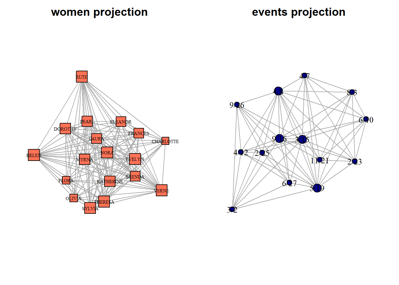
We can compute centrality values for both sets of nodes (women and events):
V(g.women)$degree = degree(g.women, mode = "all")
V(g.women)$betweenness.score <- betweenness(g.women)
V(g.women)$closeness.score <- closeness(g.women)

(g.women %>%
  asDF())$vertex %>%
  select(name, degree, betweenness.score, closeness.score) %>%
  mutate(betweenness.score = round(betweenness.score,2),
         closeness.score = round(closeness.score,2)) %>%
  arrange(desc(betweenness.score)) %>%
  kable() %>%
kable_styling(full_width = F)| name | degree | betweenness.score | closeness.score |
|---|---|---|---|
| OLIVIA | 12 | 18.53 | 0.04 |
| FLORA | 12 | 18.53 | 0.04 |
| DOROTHY | 16 | 13.02 | 0.04 |
| HELEN | 17 | 8.39 | 0.04 |
| FRANCES | 15 | 7.87 | 0.04 |
| MYRNA | 16 | 7.31 | 0.03 |
| KATHERINE | 16 | 7.31 | 0.03 |
| VERNE | 17 | 2.51 | 0.03 |
| SYLVIA | 17 | 2.51 | 0.03 |
| CHARLOTTE | 11 | 2.08 | 0.03 |
| NORA | 17 | 1.49 | 0.03 |
| ELEANOR | 15 | 0.62 | 0.03 |
| LAURA | 15 | 0.45 | 0.03 |
| BRENDA | 15 | 0.45 | 0.03 |
| EVELYN | 17 | 0.09 | 0.03 |
| THERESA | 17 | 0.09 | 0.03 |
| PEARL | 16 | 0.09 | 0.03 |
| RUTH | 17 | 0.09 | 0.03 |
By contrast, we can use tnet package to compute weighted centrality scores. To do that, we firstly need to convert our matrix to tnet format.
women_tnet <- as.tnet(women_matrix)

tnet_degree <- degree_w(women_tnet)
tnet_betweenness <- betweenness_w(women_tnet)
tnet_closeness <- closeness_w(women_tnet,
                              gconly = FALSE)

southern_women_compare <- data.frame(
  name = row.names(women_matrix),
  weighted_degree = tnet_degree[,2],
  weighted_betweenness = tnet_betweenness[,2],
  weighted_closeness = tnet_closeness[,3]) %>%

  left_join((asDF(g.women))$vertex %>%
              select(-intergraph_id))

head(southern_women_compare) %>%
  kable() %>%
kable_styling(full_width = F)| name | weighted_degree | weighted_betweenness | weighted_closeness | degree | betweenness.score | closeness.score |
|---|---|---|---|---|---|---|
| EVELYN | 17 | 4.5000000 | 1.2926019 | 17 | 0.0909091 | 0.0294118 |
| LAURA | 15 | 0.3333333 | 1.2315491 | 15 | 0.4523810 | 0.0285714 |
| THERESA | 17 | 34.3333333 | 1.4575448 | 17 | 0.0909091 | 0.0263158 |
| BRENDA | 15 | 1.5000000 | 1.2569419 | 15 | 0.4523810 | 0.0285714 |
| CHARLOTTE | 11 | 0.0000000 | 0.8642842 | 11 | 2.0833333 | 0.0285714 |
| FRANCES | 15 | 0.0000000 | 0.9477175 | 15 | 7.8690476 | 0.0357143 |
We can compare the values we got from two approaches. The values are different when plotting two types of betweenness against each other.
#southern_women_compare %>%
#  ggplot(aes(degree, weighted_degree)) +
#  geom_point() ## values are similar

southern_women_compare %>%
  ggplot(aes(betweenness.score, weighted_betweenness)) +
  geom_point() +
  geom_text_repel(aes(label = name), size = 2)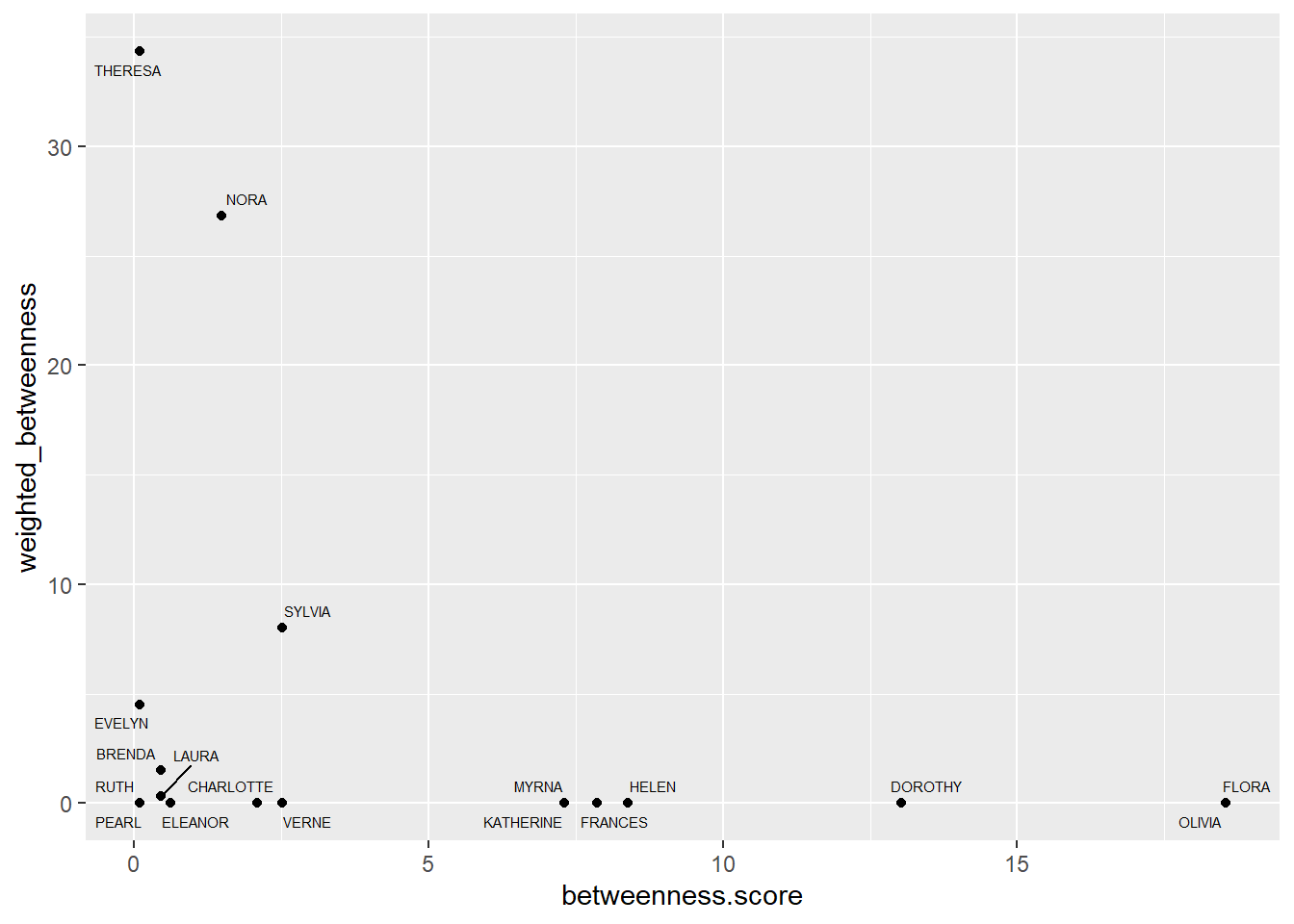
#southern_women_compare %>%
#  ggplot(aes(closeness.score, weighted_closeness)) +
#  geom_point()
Actors with the highest scores:
par(mar=c(0,0,0,0))
g.women %>%
  plot(vertex.label.cex = 0.5,
       vertex.label.color = "black",
       #vertex.size = V(g.women)$betweenness.score,
       vertex.color = ifelse(V(g.women)$name %in% c("OLIVIA", "FLORA"),
                             "coral1",
                             ifelse(V(g.women)$name %in% c("NORA", "THERESA"),

                                    "lightblue",
                                    "grey60")),
       vertex.size = V(g.women)$degree*1.5,
       vertex.shape = "square",
       layout = layout_nicely(g.women))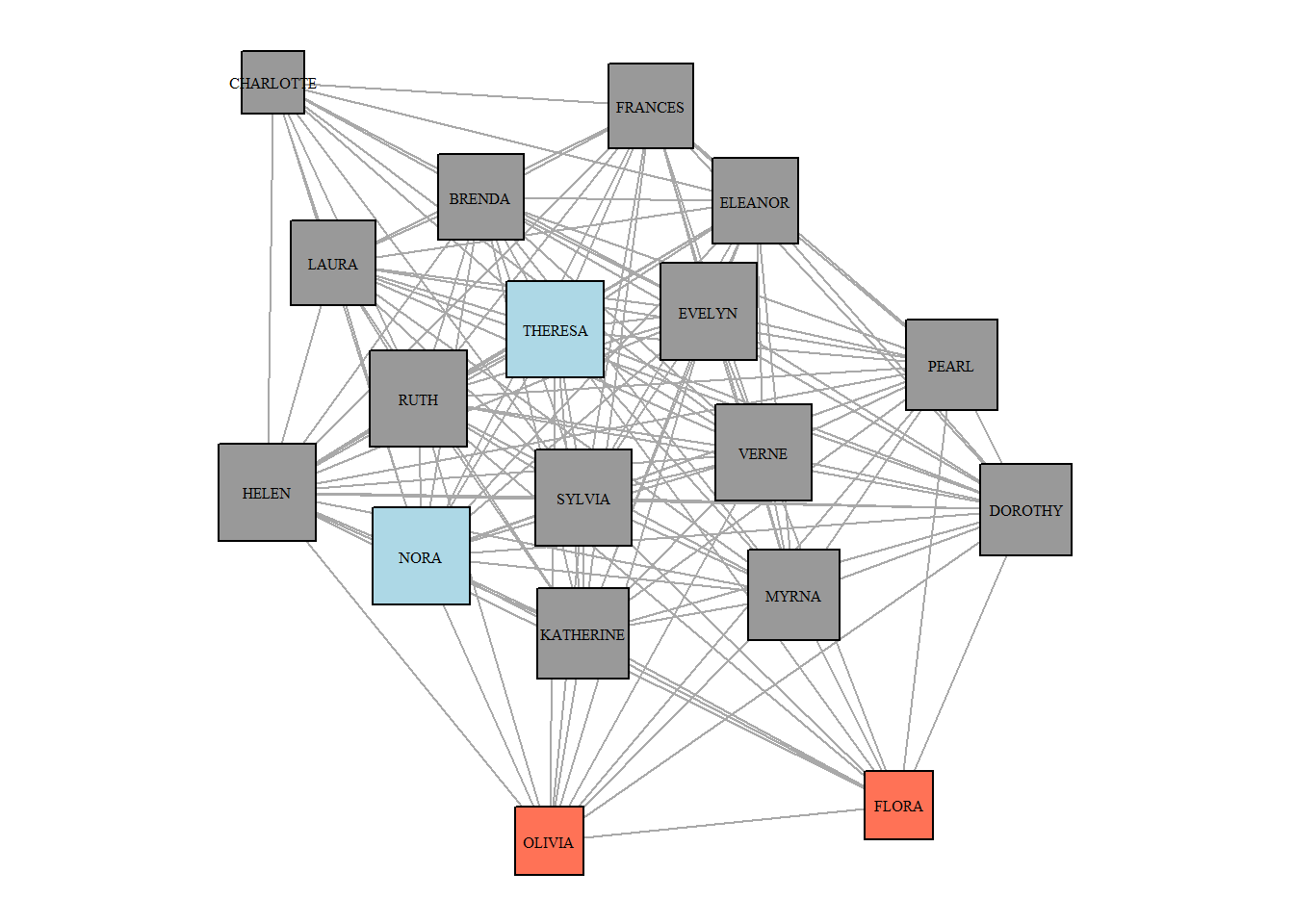
Communities in the women projection:
set.seed(42)
cl <- cluster_louvain(g.women)

V(g.women)$cl = membership(cl)

par(mar=c(0,0,0,0))
g.women %>%
  plot(vertex.label.cex = 0.5,
       vertex.label.color = "black",
       #vertex.size = V(g.women)$betweenness.score,
       vertex.size = V(g.women)$degree*1.5,
       vertex.color = ifelse(V(g.women)$cl == 1,
                             "coral1",
                             "lightblue"),
       vertex.shape = "square",
       layout = layout_nicely(g.women))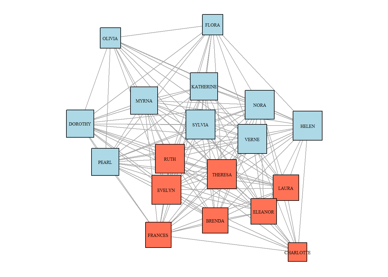
And in the matrix form (we will analyze next time):
library(blockmodeling)

class2 <- optRandomParC(M=women_matrix,
                        k = 2,
                        rep = 10,
                        approach="ss",
                        blocks="com",
                        printRep = F)
#>
#>
#> Optimization of all partitions completed
#> 1 solution(s) with minimal error = 392.3794 found.

plot(class2, main = NA)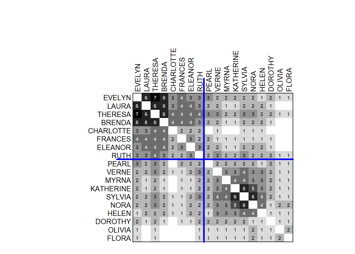
Dimensionality reduction
Dimensionality Reduction refers to the process of reducing the number of variables or dimensions in a dataset while retaining as much meaningful information as possible. This is particularly useful in exploratory data analysis, visualization, and machine learning when high-dimensional data becomes challenging to interpret or analyze.
Correspondence Analysis (CA) is a dimensionality reduction method designed for visualizing the relationships between rows and columns in a contingency table. By decomposing the chi-squared statistic of the table, it projects the data onto a lower-dimensional space, revealing patterns and associations. CA has a natural connection to the analysis of two-mode networks, as it provides a powerful framework for understanding relationships between two distinct sets of entities, much like bipartite networks.
Computation and the variation explained:
southern_women2 <- southern_women %>%
  as_biadjacency_matrix() %>%
  as.data.frame.matrix() ## 18 rows = women, 14 columns = events


library(ca)
library(factoextra)
## perform correspondence analysis
res.ca <- ca(southern_women2, graph = FALSE)

## plot with the variance explained by each dimension:
fviz_eig(res.ca)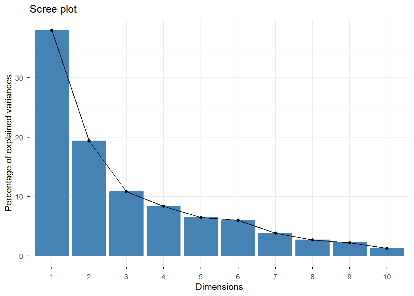
Plotting:
women.profiles <- get_ca_row(res.ca)
events.profiles <- get_ca_col(res.ca)

women.profiles$coord %>%
  data.frame() %>%
  mutate(name = row.names(.),
         type = "people") %>%

  bind_rows(events.profiles$coord %>%
              data.frame() %>%
              mutate(name = row.names(.),
                     type = "events")) %>%

  ggplot(aes(Dim.1, Dim.2, color = type)) +
  geom_point() +
  geom_text_repel(aes(label = name), size = 3) +

  scale_color_manual(values = c("darkblue", "coral1")) +
  theme(legend.position = "none")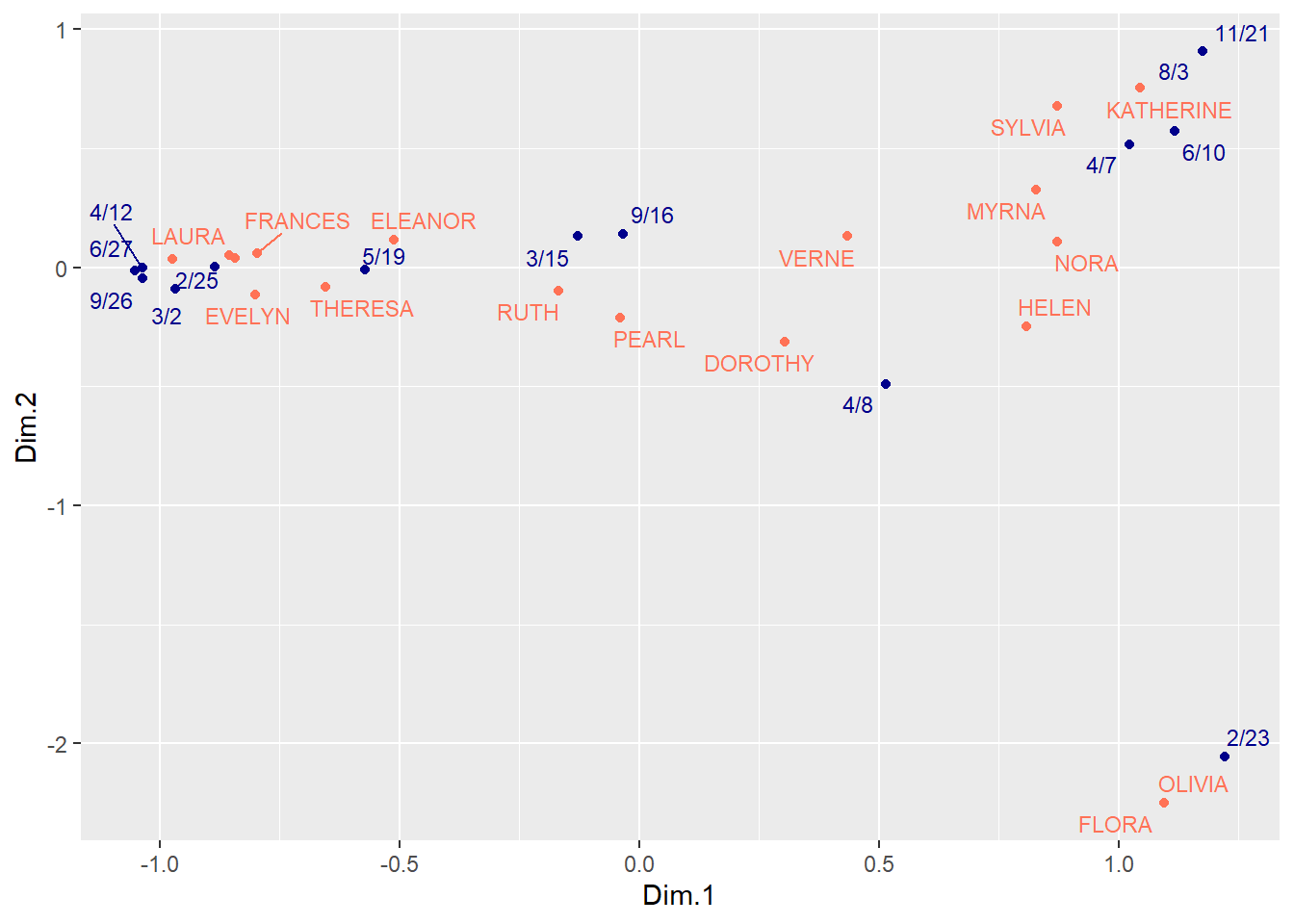
Clustering a two-mode network on cultural tastes and leisure activities
This data was collected by the group of sociology students who attended the course on “Culture and Inequality” during the spring of 2025. The goal here was to map the respondents’ perception of association between the jobs / professions and cultural preferences. The whole research strategy is inspired by:
Boltanski, L., & Thévenot, L. (1983). Finding one’s way in social space: a study based on games. Social science information, 22(4-5), 631-680.
This is an on-going project, so it is just the slice of the data. Apologies that it is in Russian.
cultural.choices <- fread("datasets/cultural.choices_table.csv")First, we need to consturct a graph object:
g <- cultural.choices %>%
count(cultural_choice, occupation_card) %>%
rename(weight = n) %>%
graph_from_data_frame(directed = F)
nodelist <- asDF(g)$edge %>%
count(V1) %>%
select(-n) %>%
left_join(asDF(g)$vertex %>%
rename(V1 = intergraph_id)) %>%
mutate(type = "choice") %>%
rename(intergraph_id = V1) %>%
bind_rows(asDF(g)$edge %>%
count(V2) %>%
select(-n) %>%
left_join(asDF(g)$vertex %>%
rename(V2 = intergraph_id)) %>%
mutate(type = "occupation") %>%
rename(intergraph_id = V2))
g <- cultural.choices %>%
count(cultural_choice, occupation_card) %>%
rename(weight = n) %>%
graph_from_data_frame(directed = F,
vertices = nodelist %>%
select(-intergraph_id))
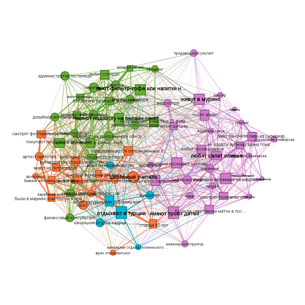
g %>%
plot(vertex.label = NA,
vertex.color = ifelse(V(g)$type == "choice",
"coral1",
"lightblue"),
vertex.shape = ifelse(V(g)$type == "choice",
"circle",
"square"))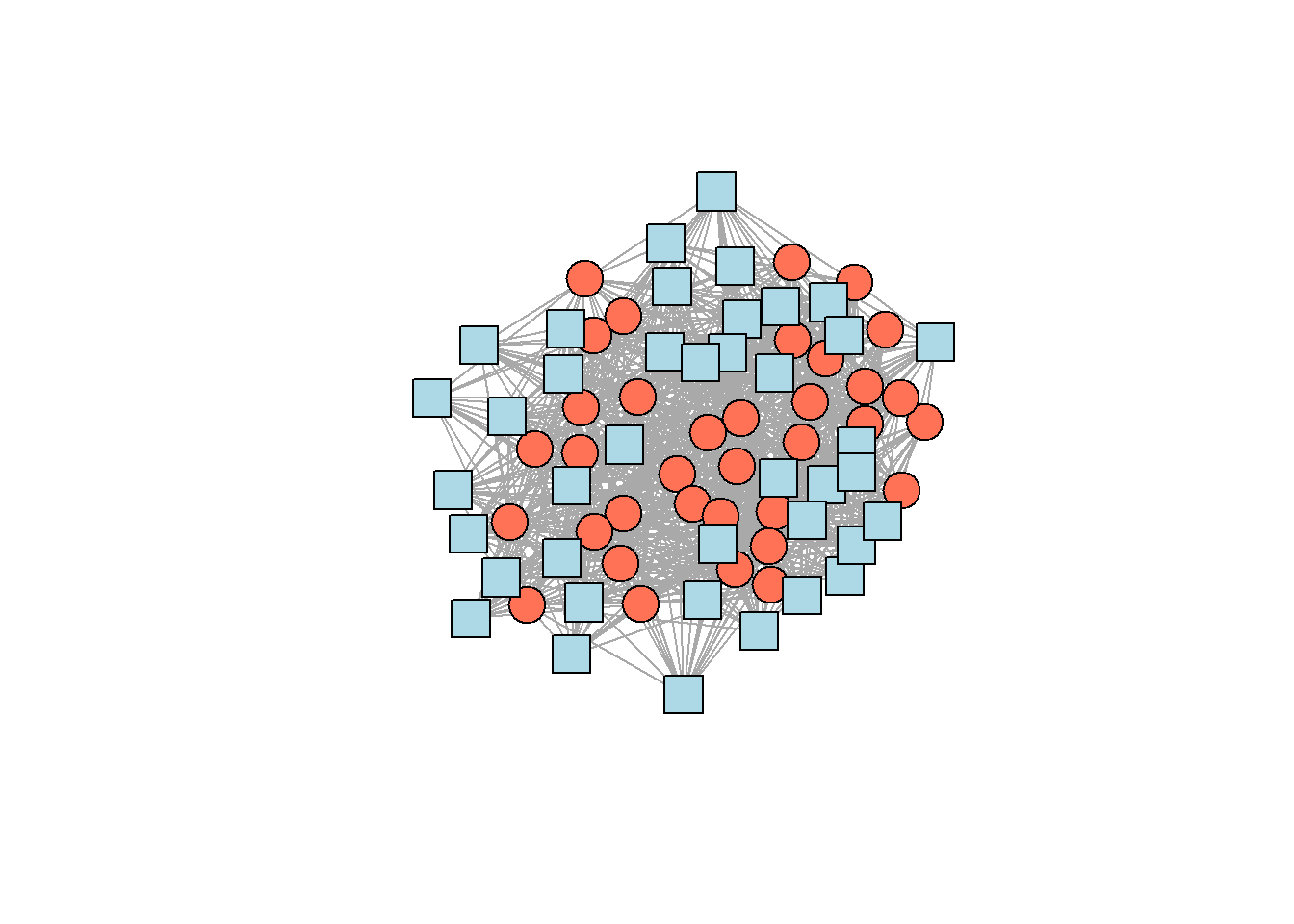
Community detection:
set.seed(42)
cl <- g %>%
  cluster_fast_greedy(weights = E(g)$weight)

  #membership() %>%
  #sizes()
cl
#> IGRAPH clustering fast greedy, groups: 4, mod: 0.29
#> + groups:
#>   $`1`
#>    [1] "бывали на каникулах в италии"
#>    [2] "были в мариинском театре в прошлом месяце"
#>    [3] "живут на петроградке"
#>    [4] "знают французский"
#>    [5] "покупают в среднем две книги в месяц"
#>    [6] "придерживаются оппозиционных политических взглядов"
#>    [7] "смотрят фестивальное кино"
#>    [8] "старше 60 лет"
#>    [9] "артист оркестра"
#>   + ... omitted several groups/vertices
Table with clusters:
V(g)$fast.greedy.cl = membership(cl)

asDF(g)$vertex %>%
  group_by(type, fast.greedy.cl) %>%
  summarise(members = toString(name)) %>%
  ungroup() %>%

  pivot_wider(names_from = "type",
              values_from = "members") %>%
  rename(`fast-greedy cluster` = fast.greedy.cl,
         choices = choice,
         occupations = occupation)
#> # A tibble: 4 × 3
#>   `fast-greedy cluster` choices                  occupations
#>   <membrshp>            <chr>                    <chr>
#> 1 1                     бывали на каникулах в и… артист орк…
#> 2 2                     были на спортивном матч… повар, про…
#> 3 3                     носят натуральную дубле… агент по н…
#> 4 4                     вегетарианцы, ежедневно… администра…

#as_image(width = 8, height = 20) -- other option
#install.packages("webshot2")
#install.packages("magick")
Overview from Gephi:
Case study: interlocking editors in Russian sociology
Read more about the data here.
load data:
vertices <- read.csv("datasets/journals_nodes.csv")
edges <- read.csv("datasets/journals_edges.csv")

mode2 <- read.csv("datasets/2mode_journals.csv")

rm(edges)
Get projections:
##########################################
## get bimodal network and projections: ##
##########################################

two.mode <- graph_from_data_frame(mode2 %>%
                                    ## get unique journal-editor couples:
                                    count(journal_name,
                                          unified_name),
                                  directed = F)

## assign bipartite mapping:
V(two.mode)$type <- bipartite_mapping(two.mode)$type

## extract projections:
bipartite_matrix <- as_biadjacency_matrix(two.mode)

journal_matrix <- bipartite_matrix %*% t(bipartite_matrix)
people_matrix <- t(bipartite_matrix) %*% bipartite_matrix

## create journals' projection:
diag(journal_matrix) <- 0
diag(people_matrix) <- 0

g_journals <- graph_from_adjacency_matrix(journal_matrix,
                                          mode = "undirected",
                                          weighted = TRUE)
g_people <- graph_from_adjacency_matrix(people_matrix,
                                          mode = "undirected",
                                          weighted = TRUE)

rm(bipartite_matrix, journal_matrix, two.mode)
Central editors:
V(g_people)$totaldegree = degree(g_people, mode = "all")
V(g_people)$betweenness.score = betweenness(g_people)

#(asDF(g_people))$vertex %>%
#  arrange(desc(totaldegree))

## better way:
mode2 %>%
  count(journal_name, unified_name) %>%
  count(unified_name) %>%
  arrange(desc(n)) %>%
  top_n(7, n) %>%
  kable() %>%
kable_styling(full_width = F)| unified_name | n |
|---|---|
| зубок юлия альбертовна | 9 |
| голенкова зинаида тихоновна | 8 |
| тощенко жан терентьевич | 8 |
| горшков михаил константинович | 7 |
| черныш михаил федорович | 6 |
| ивченков сергей григорьевич | 5 |
| каменева татьяна николаевна | 5 |
| омельченко елена леонидовна | 5 |
| погосян геворк арамович | 5 |
| скворцов николай генрихович | 5 |
| ярская-смирнова елена ростиславовна | 5 |
Central journals:
##############################
## get degree centralities: ##
##############################

V(g_journals)$degree = degree(g_journals, mode = "total")

## preview the most central journals:
(g_journals %>% asDF())$vertexes %>%
  select(-intergraph_id) %>%
  arrange(desc(degree)) %>%
  head() %>%
  kable() %>%
kable_styling(full_width = F)| name | degree |
|---|---|
| социологические исследования | 40 |
| журнал социологии и социальной антропологии | 23 |
| научный результат. социология и управление | 23 |
| теория и практика общественного развития | 23 |
| поиск: политика. обществоведение. искусство. социология. культура | 22 |
| социология | 22 |
Journal communities:
##########################
## community detection: ##
##########################

set.seed(42)
cl3 <- cluster_louvain(g_journals,
                       resolution = 0.75)

V(g_journals)$cl3 = membership(cl3)

#asDF(g_journals)

## solution preview:
set.seed(42)
par(mar=c(0,0,0,0))
plot(g_journals,
     vertex.color = ifelse(V(g_journals)$cl3 == 1,
                           "#988F2A",
                           ifelse(V(g_journals)$cl3 == 2,
                                  "coral1",
                                  "#30638E")),
     vertex.label = NA,
     vertex.size = V(g_journals)$degree * 0.6)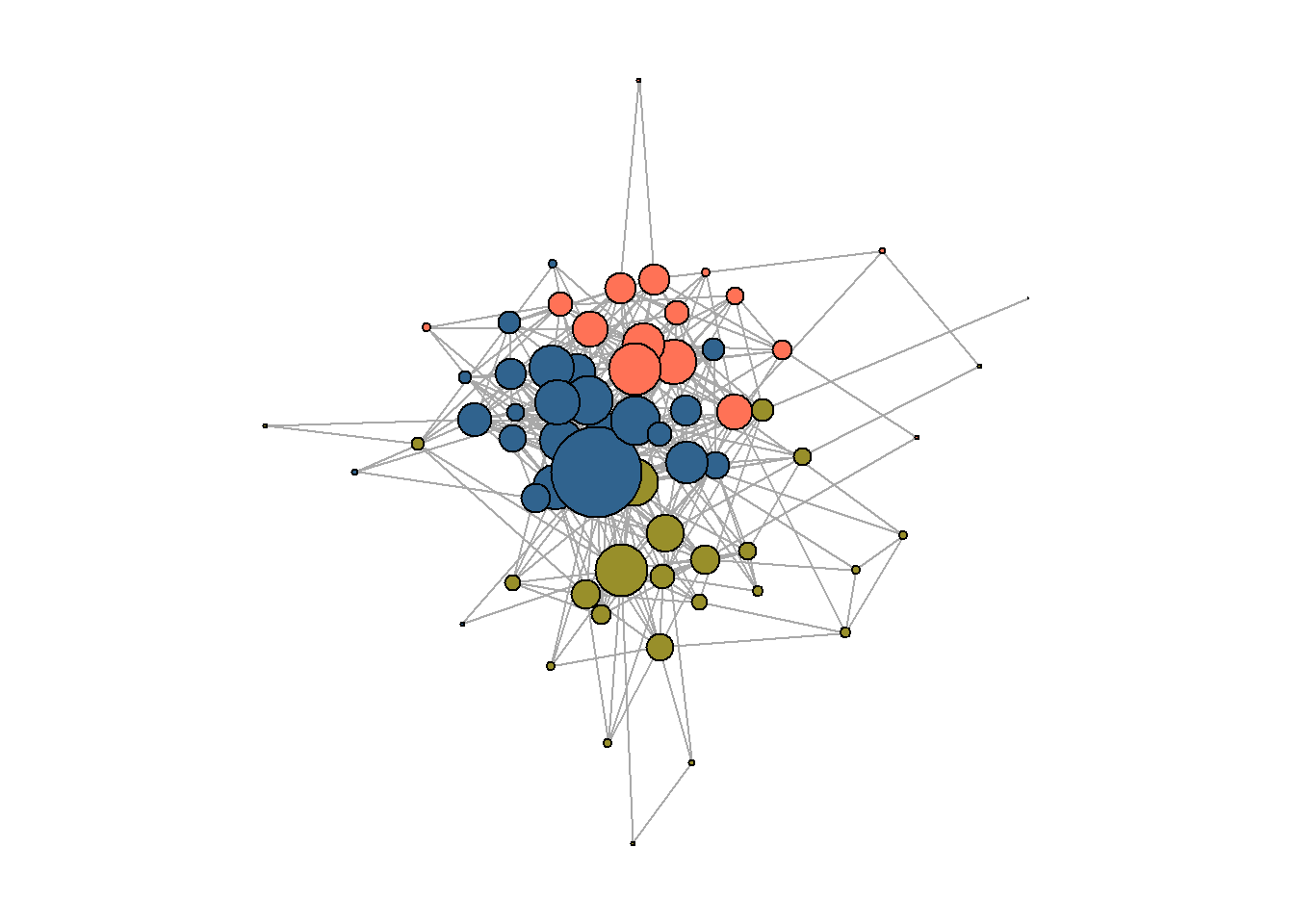
rm(cl3)Core/periphery:
#####################
## core/periphery: ##
#####################

core_peiphery <- netUtils::core_periphery(g_journals)
V(g_journals)$core_periphery = core_peiphery$vec


## solution preview:
set.seed(42)
par(mar=c(0,0,0,0))
plot(g_journals,
     vertex.color = ifelse(V(g_journals)$core_periphery == 1,
                           "lightgreen",
                           "coral1"),
     vertex.label = NA,
     vertex.size = V(g_journals)$degree * 0.6)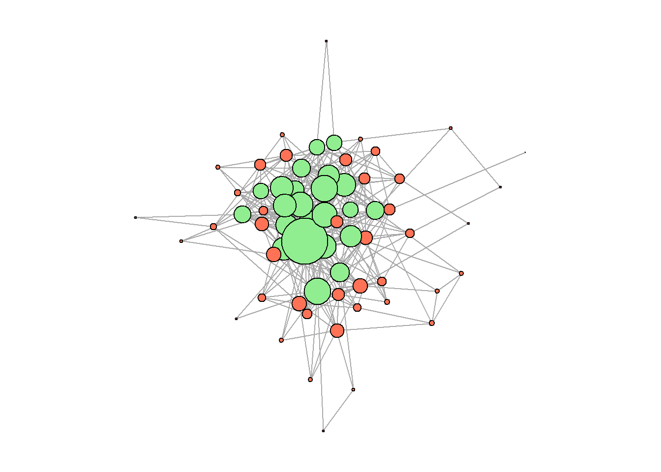
Table with partitions (core/periphery and communities):
##############################################
## table of core/periphery and communities: ##
##############################################

journals_positions <- (asDF(g_journals))$vertexes %>%
  rename(journal_name = name) %>%
  arrange(desc(degree)) %>%
  select(-intergraph_id, -degree)

## table preview:
head(journals_positions) %>%
  kable() %>%
kable_styling(full_width = F)| journal_name | cl3 | core_periphery |
|---|---|---|
| социологические исследования | 3 | 1 |
| журнал социологии и социальной антропологии | 1 | 1 |
| научный результат. социология и управление | 3 | 1 |
| теория и практика общественного развития | 2 | 1 |
| поиск: политика. обществоведение. искусство. социология. культура | 3 | 1 |
| социология | 3 | 1 |
Community properties:
###############################
## get community properties: ##
###############################

communities <- (asDF(g_journals))$vertexes %>%
  select(-intergraph_id) %>%
  rename(journal_name = name) %>%

  left_join(vertices, by = "journal_name") %>%
  mutate(cl3 = ifelse(cl3 == 1,
                      "west",
                      ifelse(cl3 == 2,
                             "east",
                             "center"))) %>%

  group_by(cl3) %>%
  summarise(mean_reference_list = mean(mean_n_references2021),
            mean_publications = mean(total_publications2021),
            mean_citations = mean(total_citations2021),

            share_foreigners = mean(share_foreigners),
            share_RAS = mean(share_ras),
            share_moscowites = mean(share_moscowite)
            ## more attributes can be calculated here. I include those which are reported among the picture.
            )

## properties' preview:
communities[1:3,1:4] %>%
  kable() %>%
kable_styling(full_width = F)| cl3 | mean_reference_list | mean_publications | mean_citations |
|---|---|---|---|
| center | 19.84167 | 72.66667 | 433.8333 |
| east | 18.92500 | 77.18750 | 303.8125 |
| west | 35.31923 | 44.84615 | 352.6154 |
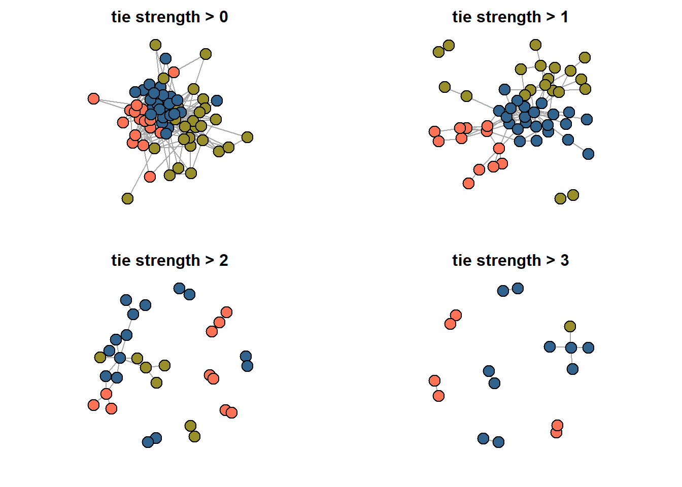
Network slices, i.e. netwroks where only “strong” ties are retained:
#######################
## reduced networks: ##
#######################

## Here, you need to run par() and loop together. To get the reduced graphs on the same picture.
## You may also need to zoom to see them (this is due to RStusio default view properties).

par(mfrow = c(2,2))

for(i in c(0:3)){

g <- g_journals %>%
  as_data_frame() %>%
  filter(weight > i) %>%
  graph_from_data_frame(directed = F)
set.seed(31)
par(mar=c(2,2,2,2))
V(g)$color <-((asDF(g))$vertexes %>%

                 left_join(journals_positions %>%
                             rename(name = journal_name)) %>%
                 mutate(cl_colors = ifelse(cl3 == 1,
                                          "#988F2A",
                                          ifelse(cl3 == 2,
                                                 "coral1",
                                                 "#30638E"))))$cl_colors
plot(g,
     vertex.label = NA,
     main = str_c("tie strength > ", i))
}
Save data to load in Gephi:
#mode2 %>%
#  count(journal_name, unified_name) %>%
#  select(-n) %>%
#  `colnames<-`(c("Source", "Target")) %>%
#  write.csv("gephi_edges.csv",
#            row.names = F)

#mode2 %>%
#  count(journal_name) %>%
#  mutate(type = "journal") %>%
#  rename(Id = journal_name) %>%

#  bind_rows(mode2 %>%
#              count(unified_name) %>%
#              mutate(type = "person") %>%
#              rename(Id = unified_name)) %>%
#  select(-n) %>%
#  mutate(name = Id) %>%
#  write.csv("gephi_nodes.csv",
#            row.names = F)
Session info:
rm(list = ls())
sessionInfo()
#> R version 4.4.3 (2025-02-28 ucrt)
#> Platform: x86_64-w64-mingw32/x64
#> Running under: Windows 10 x64 (build 19045)
#>
#> Matrix products: default
#>
#>
#> locale:
#> [1] LC_COLLATE=Russian_Russia.utf8
#> [2] LC_CTYPE=Russian_Russia.utf8
#> [3] LC_MONETARY=Russian_Russia.utf8
#> [4] LC_NUMERIC=C
#> [5] LC_TIME=Russian_Russia.utf8
#>
#> time zone: Europe/Moscow
#> tzcode source: internal
#>
#> attached base packages:
#> [1] stats     graphics  grDevices utils     datasets
#> [6] methods   base
#>
#> other attached packages:
#>  [1] data.table_1.17.8   factoextra_1.0.7
#>  [3] ca_0.71.1           blockmodeling_1.1.8
#>  [5] kableExtra_1.4.0    ggrepel_0.9.6
#>  [7] tnet_3.0.16         survival_3.8-3
#>  [9] networkdata_0.2.2   netUtils_0.8.3
#> [11] manynet_1.6.1       intergraph_2.0-4
#> [13] igraph_2.1.4        lubridate_1.9.4
#> [15] forcats_1.0.0       stringr_1.5.1
#> [17] dplyr_1.1.4         purrr_1.0.4
#> [19] readr_2.1.5         tidyr_1.3.1
#> [21] tibble_3.2.1        ggplot2_4.0.0
#> [23] tidyverse_2.0.0
#>
#> loaded via a namespace (and not attached):
#>  [1] gtable_0.3.6          xfun_0.51
#>  [3] bslib_0.9.0           lattice_0.22-6
#>  [5] tzdb_0.5.0            vctrs_0.6.5
#>  [7] tools_4.4.3           generics_0.1.4
#>  [9] parallel_4.4.3        pkgconfig_2.0.3
#> [11] Matrix_1.7-2          RColorBrewer_1.1-3
#> [13] S7_0.2.0              lifecycle_1.0.4
#> [15] compiler_4.4.3        farver_2.1.2
#> [17] codetools_0.2-20      htmltools_0.5.8.1
#> [19] sass_0.4.10           yaml_2.3.10
#> [21] pillar_1.11.1         jquerylib_0.1.4
#> [23] cachem_1.1.0          network_1.19.0
#> [25] tidyselect_1.2.1      digest_0.6.37
#> [27] stringi_1.8.4         bookdown_0.45
#> [29] splines_4.4.3         fastmap_1.2.0
#> [31] grid_4.4.3            cli_3.6.4
#> [33] magrittr_2.0.3        tidygraph_1.3.1
#> [35] withr_3.0.2           scales_1.4.0
#> [37] timechange_0.3.0      rmarkdown_2.30
#> [39] hms_1.1.3             memoise_2.0.1
#> [41] coda_0.19-4.1         evaluate_1.0.5
#> [43] knitr_1.50            viridisLite_0.4.2
#> [45] rlang_1.1.5           downlit_0.4.4
#> [47] Rcpp_1.0.14           glue_1.8.0
#> [49] xml2_1.5.0            svglite_2.1.3
#> [51] rstudioapi_0.17.1     jsonlite_2.0.0
#> [53] R6_2.6.1              statnet.common_4.11.0
#> [55] systemfonts_1.3.1     fs_1.6.6
Home assignment 4
The goal of this assignment is to analyze the structure and relationships within a two-mode network, understand its properties, and derive meaningful conclusions based on the patterns observed. Choose a dataset you like:
data you find/construct by your own (github, google, etc.)
Describe the network: who/what are the nodes? Vizualize it the way you prefer (in R or in Gephi, do not forget about different layouts possible). Select the mode of analysis: choose to work with either two-mode network or one-mode projections. In the second scenario, provide vizualizations of both projections. Discuss whether you want to work with one specific projection or not. Do the analysis you consider relevant: compute centrality measures, search for communities, core/periphery, etc.
Format: word/pdf/html. If you construct your document from R, make sure it is formatted nicely (no long outputs printed, etc.) Deadline - before your next class.