2 - centrality measures
The notes below accompany the second lecture of the course. It might be a good idea to consult the lecture slides as well, as some technical details and examples are discussed there.
Definitions of centrality measures & how to calculate them
Although there is a large variety of centrality measures out there, today we will focus on 4 core measures we have covered in class. These are:
degree centrality,
betweenness centrality,
closeness centrality,
eigenvector centrality.
The definitions are embedded in the following text as well.
The picture below borrowed form here summarizes the differences between these measures:
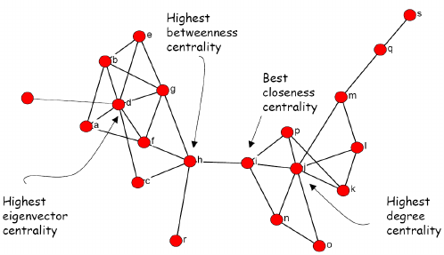
Towards the end of the last seminar, we worked with 3 types of relations among lawyers. Below, I illustrate all 4 centrality measures on these graphs. The next section covers a potentially interesting source of bibliometric (thus network) data and applications of today’s material to its analysis.
First, we need to load the libraries:
library(tidyverse)  ## general R workflow
library(igraph)     ## general network workflow
library(intergraph) ## converse from igraph to dfs
library(manynet)    ## source of lawyers' data

library(openalexR)  ## to query openalex
library(ggpmisc)    ## plotting
library(plotly)     ## interactive plotting
Second, we need to construct the lawyers’ networks (advice, friendship, and coworking) as we did it last time:
## load:
lawfirm <- manynet::ison_lawfirm

## nodelist:
nodelist <- (lawfirm %>%
  asDF())$vertexes

## edgelist:
edgelist <- (lawfirm %>%
  asDF())$edge

## divide into three networks:

## 1. advice network:
g.advice <- edgelist %>%
  filter(type == "advice") %>%
  graph_from_data_frame(vertices = nodelist,
                        directed = T)

## 2. cowork network:
g.cowork <- edgelist %>%
  filter(type == "cowork") %>%
  graph_from_data_frame(vertices = nodelist,
                        directed = T)

## 3. friendship network:
g.friends <- edgelist %>%
  filter(type == "friends") %>%
  graph_from_data_frame(vertices = nodelist,
                        directed = T)
Now, we can calculate the centrality measures.
Degree centrality stands for the number of ties that involve a given node. It is particularly meaningful for identifying popular or well-connected actors. There are various adjustments to this simple definition depending on the type of edges in your network:
total degree centrality (for undirected networks),
in-degree and out-degree centrality (for directed networks, the sum of received and sent ties respectively),
weighted degree centrality (the sum of weights of the involved ties; can be applied to the directed networks as well).
Here, as we are dealing with directed networks (ties are not necessary symmetric), we would calculate (1) in-degree and (2) out-degree centrality values. For educational purposes, I also compute (3) total degree.
The type of measure you want to get is specified via “mode” argument in degree() function from igraph package. The computations in the chunk below are done for all 3 networks.
For weighted degree centrality, use strength() function from igraph.
## in-degree:
V(g.advice)$indegree = degree(g.advice, mode = "in")
V(g.cowork)$indegree = degree(g.cowork, mode = "in")
V(g.friends)$indegree = degree(g.friends, mode = "in")

## out-degree:
V(g.advice)$outdegree = degree(g.advice, mode = "out")
V(g.cowork)$outdegree = degree(g.cowork, mode = "out")
V(g.friends)$outdegree = degree(g.friends, mode = "out")

## total-degree
## (the sum of two; for undirected networks, the argument is ignored)
V(g.advice)$totaldegree = degree(g.advice, mode = "total")
V(g.cowork)$totaldegree = degree(g.cowork, mode = "total")
V(g.friends)$totaldegree = degree(g.friends, mode = "total")

#?degree() ## read more about this measure

## head of the vertex table from friendship network:
(g.friends %>%
  asDF())$vertex %>%
  head() %>%
  select(status, gender, age, indegree, outdegree, totaldegree)
#>    status gender age indegree outdegree totaldegree
#> 1 partner    man  64        5         4           9
#> 2 partner    man  62       10         4          14
#> 3 partner    man  67        4         0           4
#> 4 partner    man  59       14        15          29
#> 5 partner    man  59        5         3           8
#> 6 partner    man  55        2         0           2
The table above contains the 3 different degree values for 6 individuals from the friendship network. Note that indegree and outdegree values might be severely different from each other.
The graph below depicts these relations:
(g.friends %>%
  asDF())$vertex %>%
  ggplot(aes(indegree, outdegree)) +
  geom_point() +
  geom_abline() +
  labs(x = "indegree\n(mentioned as friend)",
       y = "outdegrgee\n(mentions as friends)",
       title = "Friendship relations in the law firm (Lazega 2001)") +
  annotate(geom = "text",
           x = 5,
           y = 19,
           label = "named more people as friends
           than they were themselves named") +
  annotate(geom = "text",
           x = 18,
           y = 3,
           label = "named less people as friends
           than they were themselves named") +
  theme(plot.title = element_text(face="bold"))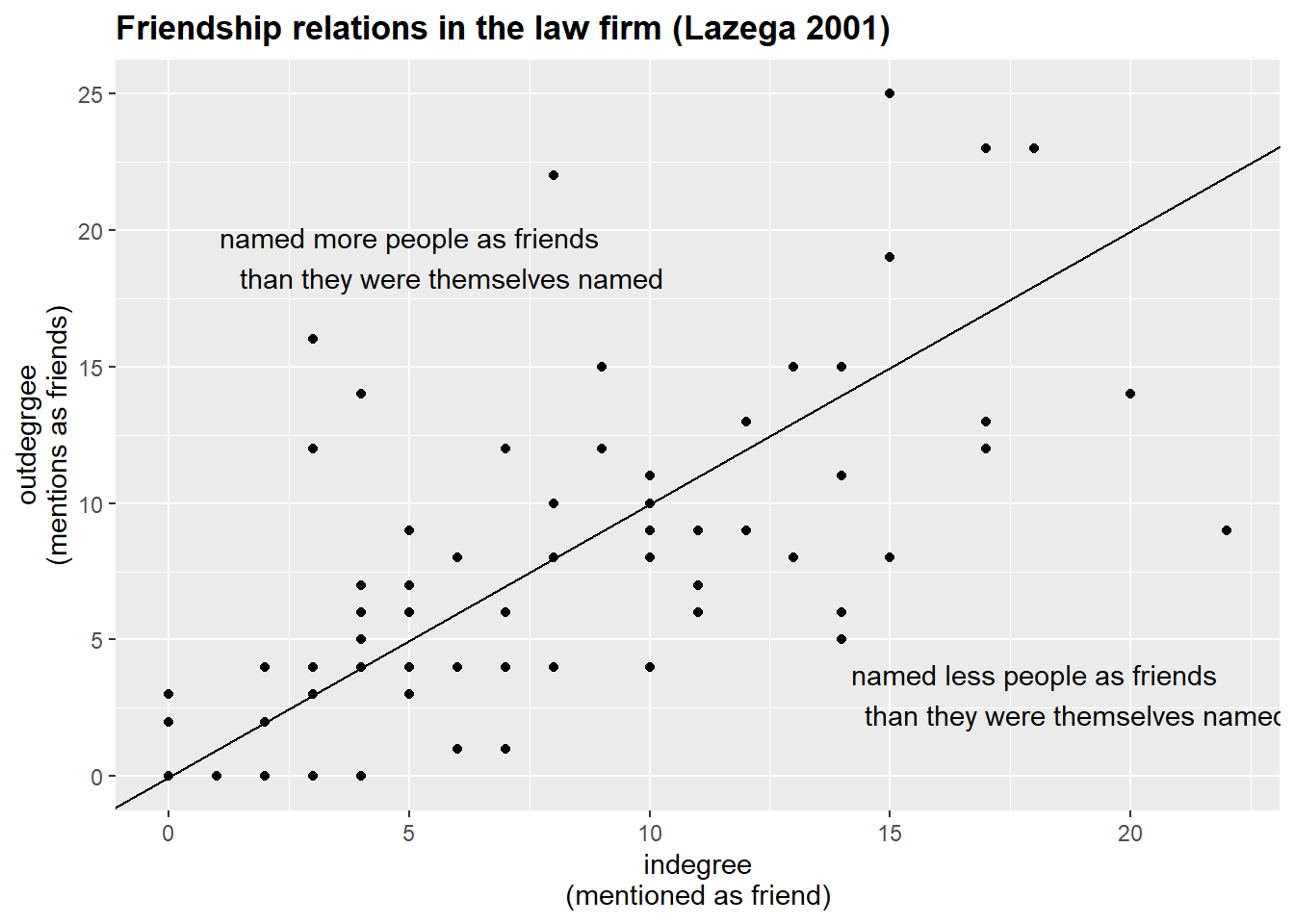
Next, let’s calculate the closeness centrality, i.e. the length of the average shortest path between a node and all other nodes in the network. In other words, it measures how quickly a node can reach all other nodes in the network. It can be valuable for identifying nodes that can rapidly disseminate information, like central offices in corporate structures.
Note that igraph offers you the normalized and inverted values, so, we need to interpret those values as the inverse of the mean distance of each node to all other nodes that the focal node can reach.
Also, in directed graphs, we need to specify the mode = "out" argument to get the desired values.
Isolates are assigned an NA value.
V(g.advice)$closeness.centrality = closeness(g.advice,
                                             mode = "out",
                                             normalized = T)
V(g.cowork)$closeness.centrality = closeness(g.cowork,
                                             mode = "out",
                                             normalized = T)
V(g.friends)$closeness.centrality = closeness(g.friends,
                                             mode = "out",
                                             normalized = T)

#?closeness() ## read more about this measure

(g.friends %>%
  asDF())$vertex %>%
  select(status, gender, age, totaldegree, closeness.centrality) %>%
  arrange(desc(closeness.centrality)) %>%
  head()
#>      status gender age totaldegree closeness.centrality
#> 1 associate    man  28          30            0.5641026
#> 2   partner    man  34          40            0.5546218
#> 3   partner    man  44          40            0.5322581
#> 4 associate    man  43          19            0.5238095
#> 5   partner    man  50          41            0.4962406
#> 6 associate    man  31          24            0.4962406
In the table above, I have filtered the data to show the lawyers with the largest values of closeness centrality. These people have extreme values of total degree centrality, so, it is relatively easy for these people to get to others.
Finally, here are the computations for betweenness centrality and eigenvector centrality. The former measures how often a node lies on the shortest paths between other nodes, indicating its potential for controlling information flow. Calculated with igraph::betweenness(), it identifies bridges or brokers in networks (e.g., think of transportation hubs or third parties managing negotiations). The eigenvector centrality, instead, assesses a node’s influence based on both its connections and the importance of those connections, capturing the concept that connecting to well-connected others benefits one’s needs. Notice that for igraph::eigen_centrality() we need to refer to vector element from the output to get the values.
## betweenness:
V(g.advice)$betweenness.centrality = betweenness(g.advice)
V(g.cowork)$betweenness.centrality = betweenness(g.cowork)
V(g.friends)$betweenness.centrality = betweenness(g.friends)

## eigenvector:
V(g.advice)$eigen.centrality = eigen_centrality(g.advice)$vector
V(g.cowork)$eigen.centrality = eigen_centrality(g.cowork)$vector
V(g.friends)$eigen.centrality = eigen_centrality(g.friends)$vector
Now we can compare different values of centrality. First, we need to get the full dataset with the computed values.
nodelist.advice <- (g.advice %>%
  asDF())$vertex
nodelist.friends <- (g.friends %>%
  asDF())$vertex
nodelist.cowork <- (g.cowork %>%
  asDF())$vertex

head(nodelist.advice) %>%
  select(-intergraph_id, -name)
#>    status gender   office seniority age   practice
#> 1 partner    man   Boston        31  64 litigation
#> 2 partner    man   Boston        32  62  corporate
#> 3 partner    man Hartford        13  67 litigation
#> 4 partner    man   Boston        31  59  corporate
#> 5 partner    man Hartford        31  59 litigation
#> 6 partner    man Hartford        29  55 litigation
#>         school indegree outdegree totaldegree
#> 1 Harvard/Yale       22         3          25
#> 2 Harvard/Yale       23         7          30
#> 3 Harvard/Yale        8         7          15
#> 4        Other       19        17          36
#> 5        UConn       17         4          21
#> 6 Harvard/Yale       21         0          21
#>   closeness.centrality betweenness.centrality
#> 1            0.3571429               42.66664
#> 2            0.4062500               48.74555
#> 3            0.4193548               24.02323
#> 4            0.4779412               64.64551
#> 5            0.3080569               21.42334
#> 6                  NaN                0.00000
#>   eigen.centrality
#> 1        0.4422204
#> 2        0.5168263
#> 3        0.2371035
#> 4        0.6679828
#> 5        0.2657700
#> 6        0.3304243
Let’s proceed with checking the correlations among the computed measures in one of the networks:
#install.packages("corrplot")
library(corrplot)

## alternatively, use `Hmsic` library to get p-values
## for our correlation scores. That would be more accurate.

nodelist.advice %>%
  select(indegree, outdegree,
         totaldegree, closeness.centrality,
         betweenness.centrality, eigen.centrality) %>%
  cor(use = "complete.obs") %>% ## the argument ignores NAs
  round(2) %>%
  corrplot(.,
           type = "upper",
           method="number",
           order = "hclust",
           tl.col = "black",
           tl.srt = 45)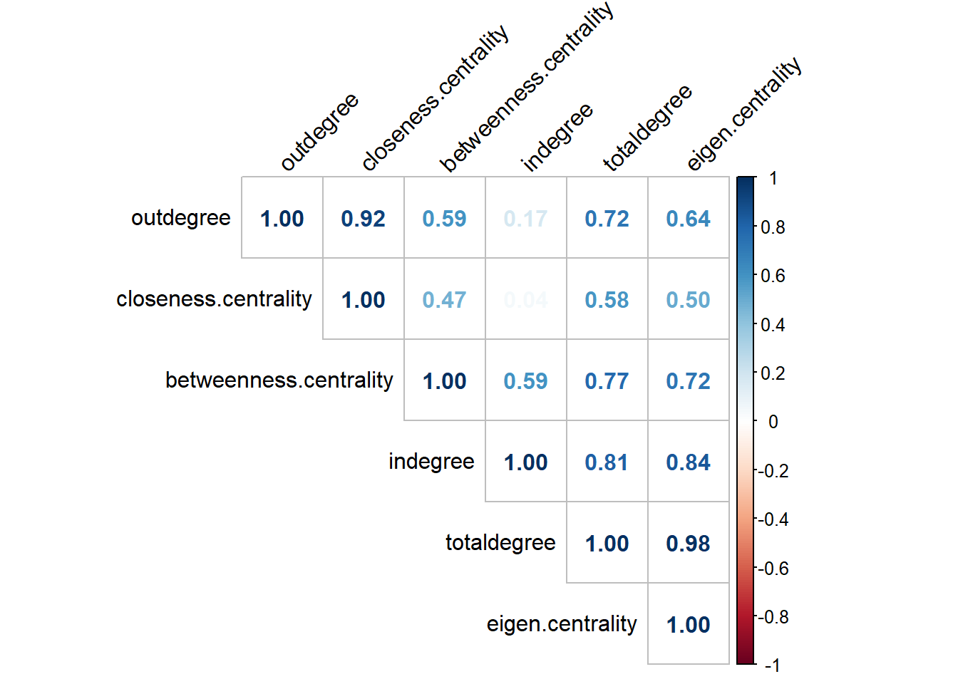
The graph shows that almost all values are highly correlated. That is to be expected when we work with the majority of networks.
The next example of analysis comes from the previous code I shared with you:
nodelist.advice %>%

  ggplot(aes(seniority, indegree)) +
  geom_point() +
  geom_smooth() +
  labs(y = "in-degree in advice network\n",
       subtitle = "The effect of seniority on centrality in advice network
       is diminished after 10+ years of work") +
  theme_minimal() +
  theme(plot.subtitle = element_text(face='bold'))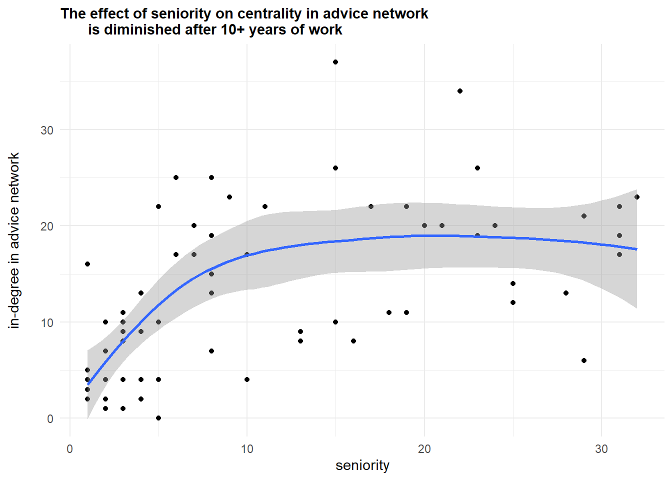
Further, let’s compare the top-10 lists according to indegree and betweenness centralities in coworkers’ network:
nodelist.cowork %>%
  arrange(desc(totaldegree)) %>%
  top_n(10, totaldegree) %>%
  mutate(totaldegree_top = str_c(name, " (", totaldegree, ")")) %>%
  select(totaldegree_top) %>%

  bind_cols(nodelist.cowork %>%
  arrange(desc(betweenness.centrality)) %>%
  top_n(10, betweenness.centrality) %>%
  select(name, status, age, betweenness.centrality) %>%
  mutate(betweenness_top = str_c(name,
                                 " (",
                                 round(betweenness.centrality, 2),
                                 ")")) %>%
  select(betweenness_top)) %>%
  mutate(top = c(1:10)) %>%
  select(top, totaldegree_top, betweenness_top)
#>    top totaldegree_top betweenness_top
#> 1    1         26 (70)     22 (296.09)
#> 2    2         22 (64)     16 (265.89)
#> 3    3         24 (63)     26 (259.44)
#> 4    4         16 (58)     24 (244.36)
#> 5    5         19 (57)     19 (210.35)
#> 6    6         15 (56)     28 (205.24)
#> 7    7         17 (53)     15 (200.38)
#> 8    8         28 (52)     31 (185.29)
#> 9    9         31 (51)     17 (165.92)
#> 10  10          4 (48)     13 (150.21)
Though the majority of actors occur in both lists (26, 22, 24, 16, 19, 15, 17, 28, 31), there node “13” seems to possess some gatekeeping potential. Finally, we can visualize these networks.
To avoid dealing with arrows, I convert the networks to undirected mode (this procedure is purely for plotting purposes).
par(mfrow = c(2,2))
set.seed(31)
par(mar=c(0,0,1,0))
g.cowork %>%
  as_undirected() %>%
  plot(vertex.color = "lightblue",
       vertex.size = V(g.cowork)$betweenness.centrality/15,
       vertex.label = NA,
       edge.size = 1,
       edge.color = "black",
       main = "nodesize/distribution of betweenness",
       vertex.label.color = "black")

set.seed(31)
par(mar=c(0,0,1,0))
g.cowork %>%
  as_undirected() %>%
  plot(vertex.color = "coral1",
       vertex.size = V(g.cowork)$totaldegree/5,
       vertex.label = NA,
       edge.size = 1,
       edge.color = "black",
       main = "nodesize/distribution of degree",
       vertex.label.color = "black")


par(mar=c(3,3,3,3))

(g.cowork %>%
  asDF())$vertex %>%
  pull(betweenness.centrality) %>%
  hist(main = NULL, col = "lightblue")


par(mar=c(3,3,3,3))

#windows(width = 4, height = 3)
(g.cowork %>%
  asDF())$vertex %>%
  pull(totaldegree) %>%
  hist(main = NULL, col = "coral1")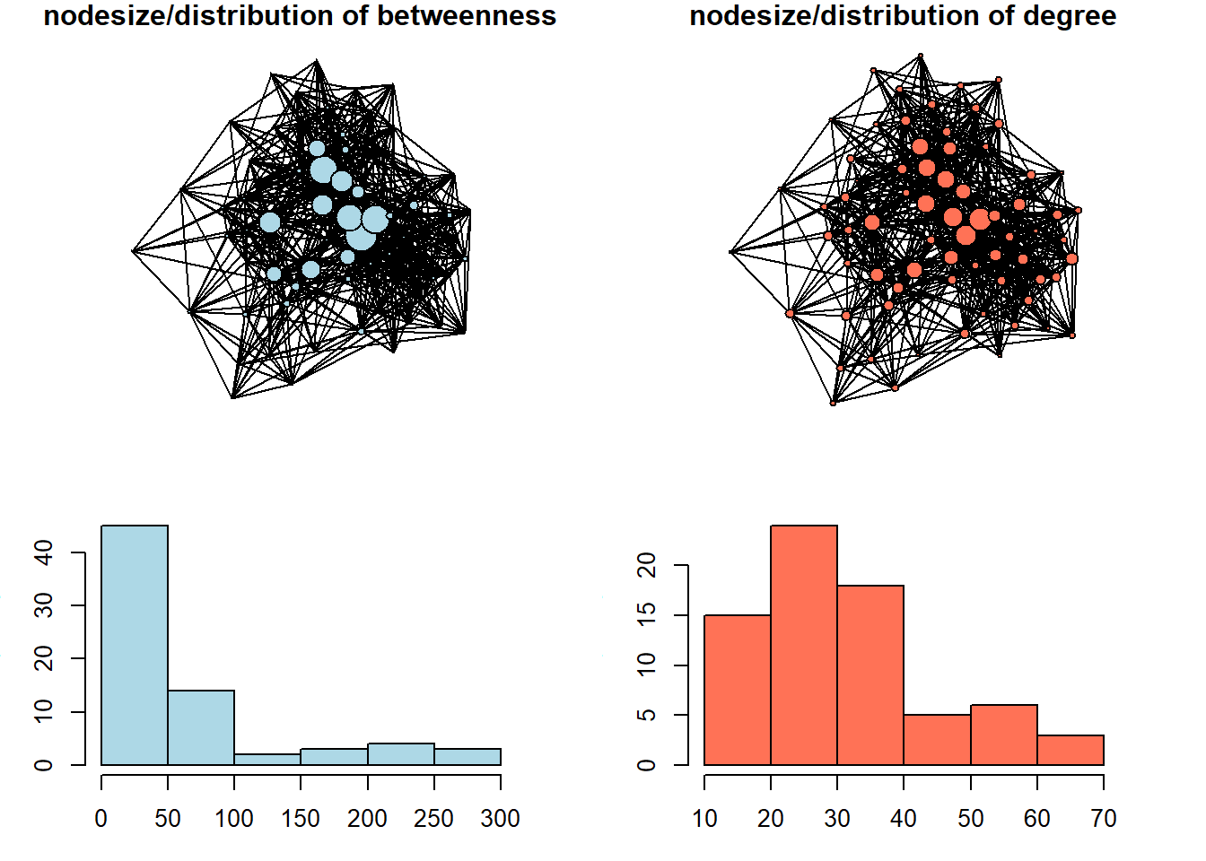
We can see here that betweenness centrality is a way more discriminating measure: most of the nodes in this network do not occur on the shortest paths between other nodes very often. In the network with size equal to degree centrality, we can see that the distribution is less severe.
Working through bibliometric example from OpenAlex data
As the topic of centrality measures is relatively straightforward, I thought it might be of some interest for you if we pick a bibliometric database for the next example, so that you would (1) get your hands on freely available scientific literature metadata, suggested by OpenAlex project, and (2) relate the ideas on centrality to bibliometric analysis. Though there are many options for the literature search nowadays, ranging from simplistic google.scholar search field to the fancy AI-tools, it might be a good idea in concrete scenarios to study the literature formally with network analysis tools. It mostly applies to clustering / community detection techniques, which we are going to covert next week, but nothing prevents us from computing centrality measures on this sorts of data as well. Obviously, there are many specialized programs developed specifically for science mapping / literature reviews (e.g. VOSviewer, CitNetExplorer, etc.), but loading, cleaning, and exploring the entire subset of literature you are interested in from R can be useful.
Currently, it is hard to access Scopus/Web of Science data (these are commonly used sources of data for scientometric studies) from Russia due to restrictions from these companies (although you still can get some metadata if you create an API key for Scopus and utilize tools like rscopus package (read documentation here), - but, remember, the output would be limited, and the speed/limits are present for this option). For this reason, we would rely on OpenAlex, - a comprehensive, freely accessible database of the global scholarly system, including millions of journal articles, authors, institutions, and research concepts. Its major advantage is that it provides a straightforward way to access and analyze citation networks and research trends for free, making it ideal for bibliometric analysis.
For our ease, there is a wonderful package called openalexR (documentation). If you are interested in the topic, you can dive into the filters’ specifications, or just follow the example suggested below. To put this simply, we need to make a search query by using multiple arguments of the function oa_fetch(), check whether we are satisfied with the output lengths, adjust our request if needed, and finally download the data.
For example, we can search for the “works” (papers, books, reviews, etc.) that contain the phrase “Sustainable Business Models” in their titles, and request just the overall number of found publications by setting the “count_only” argument to TRUE:
oa_fetch(entity = "works",
         output = "dataframe",
         display_name.search = 'Sustainable Business Models',
         count_only = T)
#>      count db_response_time_ms page per_page
#> [1,]  3812                  14    1        1
The output means that there are almost 4 thousands of works related to our query in OpenAlex. Let’s reduce this number by setting the “cited_by_count” argument to be more than 10, meaning that only works cited more than 10 times would be returned. It is our data for this demonstration.
oa_sustainable <- oa_fetch(entity = "works",
         output = "dataframe",
         display_name.search = 'Sustainable Business Models',
         cited_by_count = ">10",
         verbose = T) ## takes around 20 seconds with my internet connection
The returned data frame contains 897 rows (articles, books, etc.) and 38 columns (data on our works, ranging from titles and publication years to cited references, which is of primary interest to us as network analysts). Below is the complete list of variables exported from OpenAlex:
oa_sustainable %>%
  colnames()
#>  [1] "id"
#>  [2] "title"
#>  [3] "display_name"
#>  [4] "author"
#>  [5] "ab"
#>  [6] "publication_date"
#>  [7] "relevance_score"
#>  [8] "so"
#>  [9] "so_id"
#> [10] "host_organization"
#> [11] "issn_l"
#> [12] "url"
#> [13] "pdf_url"
#> [14] "license"
#> [15] "version"
#> [16] "first_page"
#> [17] "last_page"
#> [18] "volume"
#> [19] "issue"
#> [20] "is_oa"
#> [21] "is_oa_anywhere"
#> [22] "oa_status"
#> [23] "oa_url"
#> [24] "any_repository_has_fulltext"
#> [25] "language"
#> [26] "grants"
#> [27] "cited_by_count"
#> [28] "counts_by_year"
#> [29] "publication_year"
#> [30] "ids"
#> [31] "doi"
#> [32] "type"
#> [33] "referenced_works"
#> [34] "related_works"
#> [35] "is_paratext"
#> [36] "is_retracted"
#> [37] "concepts"
#> [38] "topics"
We can start by taking a look at the time distribution of our articles:
oa_sustainable %>%
  ggplot(aes(publication_year)) +
  geom_histogram(bins = 20) +
  theme_minimal() +
  labs(title = '**OpenAlex works (*897*) on "Sustainable Business Models"**',
       subtitle = "works with > 10 citations are retained") +
  theme(plot.title = ggtext::element_markdown())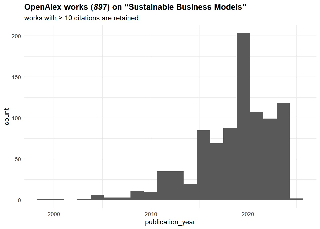
It seems that the topic is on the rise since the mid-2010s. Let’s construct now a citation network from these sources. To do that, we need to work with “referenced_works” column, which basically lists sources referenced by a given work. Surely, it might not be ideal for all works (e.g., Russian sources are often poorly represented (in terms of metadata) in OpenAlex), but it should be fine for our purposes.
We start by getting an edgelist of citations. Note that we limit our sample to just those works covered by our search query, meaning that “cited_by_count” values (number of documents citing a work) should not match the in-degree centrality values that we are going to compute. To exclude all external (not from our sample) works, we can filter the “referenced_works” by “id” column:
oa_edges <- oa_sustainable %>%
  select(id, referenced_works) %>%
  unnest(referenced_works) %>%
  mutate(referenced_works = str_squish(
    str_remove_all(referenced_works,
                   "https\\:\\/\\/openalex\\.org\\/"))) %>%

  filter(referenced_works %in% str_squish(
    str_remove_all(oa_sustainable$id,
                   "https\\:\\/\\/openalex\\.org\\/"))) %>%

  mutate(id = str_squish(
    str_remove_all(id,
                   "https\\:\\/\\/openalex\\.org\\/"))) %>%
  `colnames<-`(c("from", "to"))

oa_edges %>%
  head()
#> # A tibble: 6 × 2
#>   from        to
#>   <chr>       <chr>
#> 1 W1966481002 W1998953777
#> 2 W1966481002 W2021655427
#> 3 W1966481002 W2056268536
#> 4 W1966481002 W1568766594
#> 5 W1966481002 W1510372480
#> 6 W1966481002 W2145720744
We proceed by constructing a network and producing an initial visualization:
oa_g <- oa_edges %>%
  graph_from_data_frame(directed = T) %>%
  simplify()

set.seed(32)
par(mar=c(0,0,0,0))
oa_g %>%
  plot(vertex.label = NA,
       vertex.size = 3,
       vertex.color = "coral1",
       edge.color = "black",
       edge.size = 1)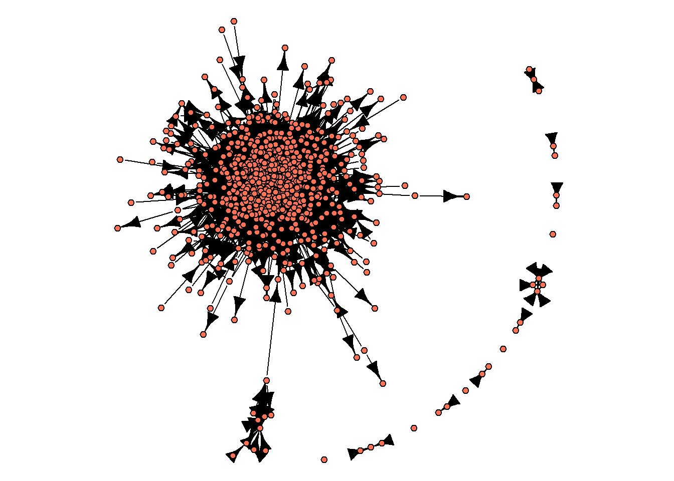
As you can see from this image, there is no single network, - instead, there are some isolated groups of nodes, with one of these sub-networks including a large proportion of networks’ nodes. These sub-networks are called “components”. We can get info on the number of components in an igraph object with components() function:
components(oa_g) %>%
  str()
#> List of 3
#>  $ membership: Named num [1:724] 1 1 1 1 1 1 1 1 1 1 ...
#>   ..- attr(*, "names")= chr [1:724] "W1966481002" "W2810801192" "W2549080287" "W2437319536" ...
#>  $ csize     : num [1:14] 699 3 4 2 3 2 1 2 2 1 ...
#>  $ no        : num 14
This output means that:
there are 724 nodes in our network (this number is below number of rows in “oa_sustainable”, the data frame we got from OpenAlex, due to missing values in “referenced_works” column, and the removal of nodes that do not link to other nodes in our literature base),
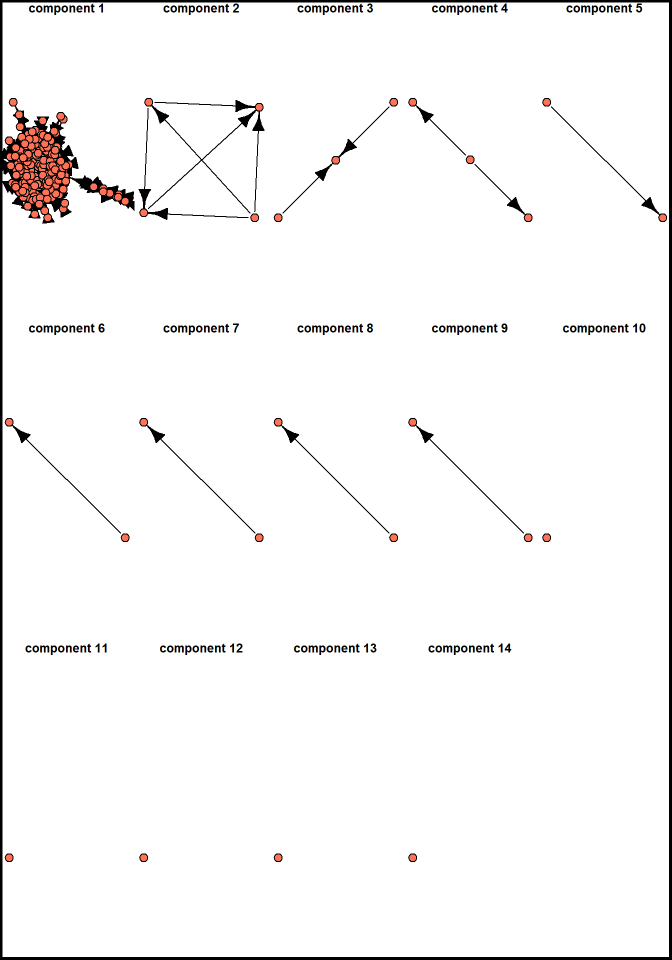
there are 14 components (clusters, sub-graphs, etc.) in our network, with the largest of them including 699 nodes (thus being 96.5% of network nodes).
A usual procedure in such cases in network analysis is to describe the network structure (number of small components, the distribution of nodes among them) and continue by analyzing the largest component in details. Before doing this, we can assign membership attribute to our nodes and plot these sub-networks separately:
V(oa_g)$component.id = components(oa_g)$membership
components.freq <- asDF(oa_g)$vertex %>%
  count(component.id) %>%
  arrange(desc(n))

set.seed(32)
par(mfrow = c(3,5))

for(i in c(1:nrow(components.freq))){

  par(mar=c(0,0,0,0))
  induced_subgraph(oa_g,
                   asDF(oa_g)$vertex %>%
                     filter(component.id == components.freq[i,1]) %>%
                     pull(name)) %>%

    plot(vertex.label = NA,
         vertex.color = "coral1",
         edge.color = "black",
         main = str_c("\ncomponent ", i))

  box("outer", col="black", lwd = 5)

}
Let’s extract the largest (first) component from the already existing igraph object. To do that, we need to get the list of nodes involved in this component:
vertices_in_largest_component = asDF(oa_g)$vertex %>%
  filter(component.id == 1) %>%
  pull(name)

oa_g.biggest <- induced_subgraph(oa_g, vertices_in_largest_component)
oa_g.biggest
#> IGRAPH 6b1cc81 DN-- 699 5476 --
#> + attr: name (v/c), component.id (v/n)
#> + edges from 6b1cc81 (vertex names):
#>  [1] W1966481002->W2021655427 W1966481002->W2056268536
#>  [3] W1966481002->W1568766594 W1966481002->W1510372480
#>  [5] W1966481002->W2105843871 W1966481002->W1998953777
#>  [7] W1966481002->W2145720744 W1966481002->W2099913992
#>  [9] W1966481002->W2283181400 W2810801192->W1966481002
#> [11] W2810801192->W2549080287 W2810801192->W2437319536
#> [13] W2810801192->W2021655427 W2810801192->W2149296970
#> [15] W2810801192->W2887423052 W2810801192->W2481733813
#> + ... omitted several edges
Finally, this is a network we would analyze from the perspective of centrality measures. It contains 699 nodes (works) and 5,476 edges between them, - and this is a directed network (direction indicates referencing of a previous work). We can start by calculating all the centrality measures:
V(oa_g.biggest)$indegree.centrality = degree(oa_g.biggest,
                                   mode = "in")
V(oa_g.biggest)$closeness.centrality = closeness(oa_g.biggest,
                                                 mode = "out",
                                                 normalized = T)
V(oa_g.biggest)$betweenness.centrality = betweenness(oa_g.biggest)
V(oa_g.biggest)$eigen.centrality = eigen_centrality(oa_g.biggest)$vector
And binding this values with the data we got from OpenAlex (publication year, total numbers of citations, document types, etc.):
oa_network_and_biblio <- (oa_g.biggest %>%
  asDF())$vertex %>%
  left_join(oa_sustainable %>%
  select(id, title, ab, so, publication_year,
         first_page, last_page, cited_by_count, type) %>%
  mutate(id = str_squish(str_remove_all(id,
                             "https\\:\\/\\/openalex\\.org\\/"))) %>%
  rename(name = id)) %>%
  select(-intergraph_id, -component.id)
The combination of network data with the attributes of the works allows to analyze how the field developed. The picture below shows the same dynamics of yearly publications as before, but it also indicates how published works were cited in this scientific domain. Note that it is different from “cited_by_count” variable, which accounts for the entire referencing (beyond publications falling in our query). When the volume of publications got large enough (and some of them got many citations), “review” appeared as a genre which can accumulate citations as well.
oa_network_and_biblio %>%
  mutate(type = ifelse(type == "article",
                       "article",
                       ifelse(type == "review",
                              "review",
                              "other"))) %>%
  ggplot(aes(publication_year, indegree.centrality, color = as.factor(type))) +
  geom_point() +
  theme_minimal() +
  labs(color = NULL,
       x = "publication year",
       y = "in-degree centrality (# of citations in corpus)",
       title = '**OpenAlex works on "Sustainable Business Models" constituting the largest component (*699*)**',
       subtitle = "works with > 10 citations are retained") +
  theme(plot.title = ggtext::element_markdown())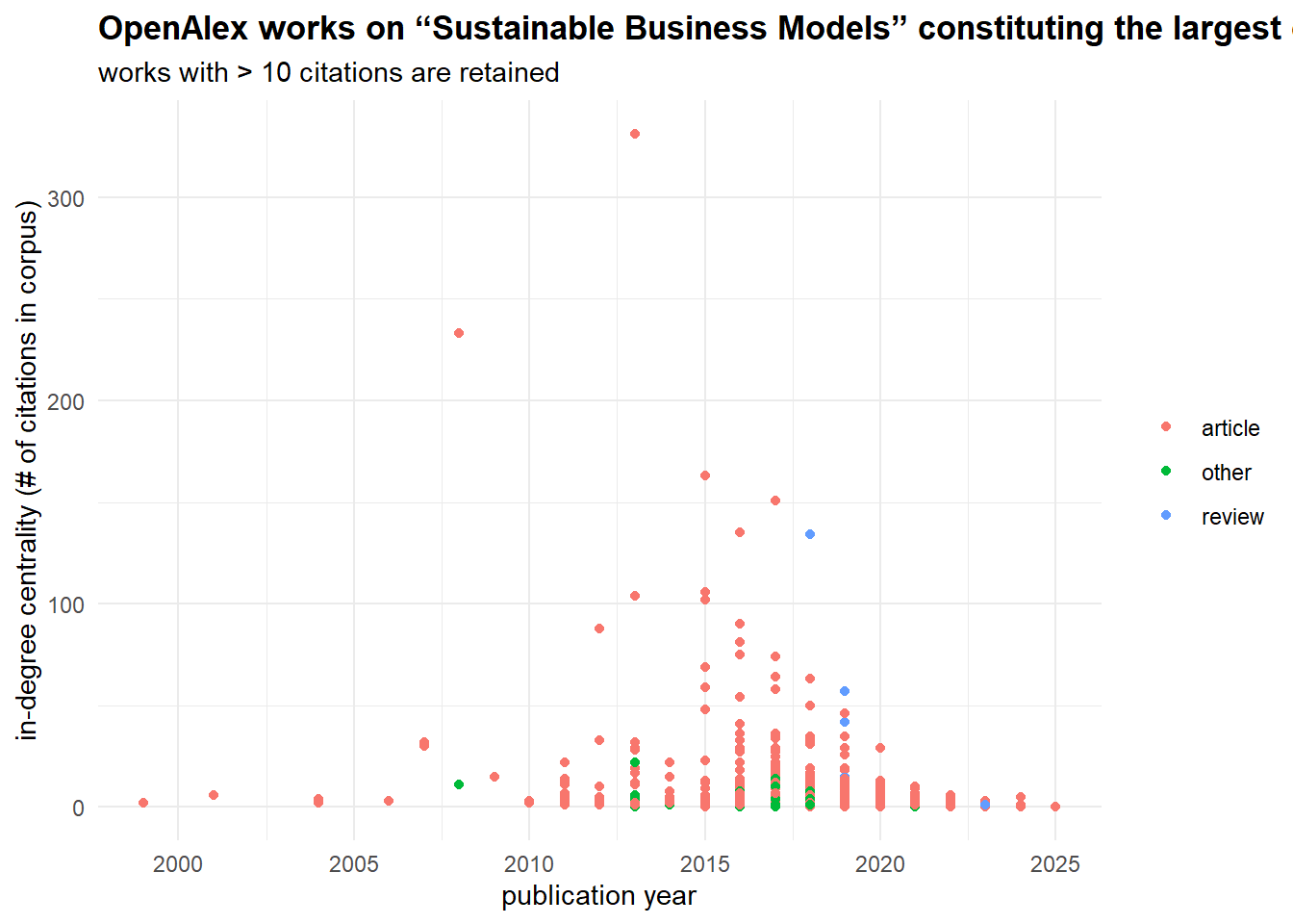
Speaking of cited_by_count papers, we can compare these scores to the network centrality metrics we have just calculated:
oa_network_and_biblio %>%
  select(name, indegree.centrality, closeness.centrality,
         betweenness.centrality, eigen.centrality,
         cited_by_count) %>%

  pivot_longer(cols = c(indegree.centrality, closeness.centrality,
                        betweenness.centrality, eigen.centrality),
               names_to = "centrality.measure",
               values_to = "centrality.value") %>%

  ggplot(aes(centrality.value, cited_by_count)) +

  #stat_poly_line() +
  #stat_poly_eq() +
  geom_point() +

  facet_wrap(~centrality.measure,
             scales = "free") +
  geom_smooth()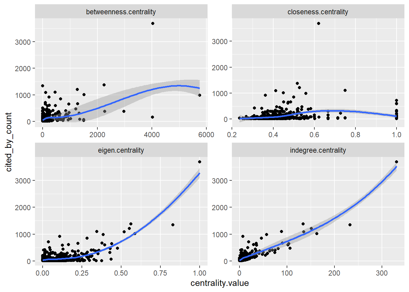
The very high correlation (0.88, p-value < 0.01) between in-degree centrality and cited_by_count is expected because they are essentially measuring the same thing: in-degree is the local citation count within our specific network. This result is expected.
The moderate correlation for eigenvector centrality (0.66, p-value < 0.01) indicates that citations from well-connected, influential papers (rather than just numerous papers) provides an additional, independent boost to a work’s total impact. The lower correlation for betweenness (0.56, p-value < 0.01) suggests that while acting as a bridge between research communities can bring some recognition, it is a less direct driver of high citation counts than simply being frequently cited. Finally, the near-zero correlation for closeness (0.13, p-value < 0.01) is common in citation networks; the speed at which a paper can reach others in the network is largely irrelevant—what matters is whether others actually cite it. The relevance of this score is also disrupted by the directed nature of our network.
By relying on centrality measures, we can differentiate locally and globally central nodes (works) and gatekeeping works, here meaning works connecting different topics / lines of research.
plot_ly(oa_network_and_biblio,
        x = ~indegree.centrality,
        y = ~betweenness.centrality,
        type = 'scatter',
        mode = 'markers',
        text = ~paste("<b>Title:</b> ", title, "<br>",
                     "<b>Publication year:</b> ", publication_year, "<br>",
                     "<b>Journal:</b> ", so, "<br>",
                     "<b>In-degree:</b> ", indegree.centrality, "<br>",
                     "<b>Betweenness:</b> ", round(betweenness.centrality, 1)),
        hoverinfo = 'text') %>%
  layout(title = "<b>Differentiating literature by citation patterns</b>",
         xaxis = list(title = "in-degree centrality"),
         yaxis = list(title = "betweenness centrality"))
Home assignment 2
You need to select a network dataset you like (check Available datasets) and analyze the most central nodes in it. To do that,
come up with 2-3 hypotheses about the central actors,
match them with the certain centrality measures we discussed in class (types of degree centrality, betweenness, etc.),
present and discuss the results the way you think is relevant. For example, you can draw the network highlighting the central nodes or present a table with various centrality scores (do not insert very large tables, include the nodes with the max./min. values or those nodes you think are important). Preferably, your hypotheses should include nodes’ variables not related to the network itself (gender, age, office, etc.). In the latter case, you can continue with distributions, scatterplots, or summary statistics table and simple regression modeling.
Whatever analysis flow you choose, reflect on your steps, results, and difficulties in text. The work can be sumbitted in word/pdf/html format (just copy tables / visualizations in the first two scenarios and comment on them).
If you want to revisit some theory, you can check the lecture by Lada Adamic or this or that pages (with R!).
Deadline - before your next class.